Short Latency Auditory Evoked Potentials
Relevant Paper
Audiologic Evaluation Working Group on Auditory Evoked Potential Measurements
Introduction
Background
The Working Group on Auditory Evoked Potential Measurements was constituted (a) to review evidence and elevate the degree of consensus existing with respect to the procedural variables and instrumentation in the application of auditory sensitivity and (b) to provide a report that is highly specific in nature and intended to be a state-of-the-science update about methodology.
In partial response to this mandate, the working group elected to develop a basic overview or tutorial focused on the short latency auditory evoked potentials (AEPs). This class of AEPs encompasses the areas of electrocochleography (ECochG) and auditory brainstem response (ABR) measurement. These potentials represent sensory or neural responses from lower levels of the auditory system. The term latency is used to describe the time of occurrence of a given potential that, for these potentials, generally falls within 10 ms of stimulus onset. This restriction in scope was made in view of the voluminous literature that has developed concerning the short latency potentials. Although rapid expansion of information continues, basic principles can be drawn from research and clinical experience with these potentials.
Scope
Short latency AEPs are popular for the electrophysiologic assessment of otology and neurologic impairment. The stability of these potentials over subject state, the relative ease with which they may be recorded, and their sensitivity to dysfunctions of the peripheral and brainstem auditory systems make them well-suited for clinical application. However, clinical application of AEP measurements requires an understanding of some procedural and subject variables.
The short latency potentials are small amplitude, far field potentials; that is, they are recorded at some distance from their sources. Sophisticated techniques are needed to measure these potentials because they are buried in a background of physical and physiological noise. Additionally, variables such as the subject's age, gender, and core temperature and the status of the outer, middle, and inner ears may predictably affect these responses. The ways in which these factors influence the measurement, analysis, and/or interpretation of the short latency potentials are discussed in this report.
The intent of this document is not to mandate a set of standards for the measurement and evaluation of short latency AEPs. Rather the objective is to present a background of information that the working group believes to be requisite for a basic understanding of these measures. The audiologist wishing to enter this area of clinical study is encouraged to take appropriate courses and seek supervised clinical experiences. Additionally, several texts on this topic have appeared that may be useful references (see Glattke, 1983; Hood & Berlin, 1986; Jacobson, 1985; Moore, 1983).
The tutorial is divided into three major sections. The first, Instrumentation—Basic Principles, presents instrumentation for both the stimulus generation and the recording and analysis methods that are common to noninvasive ECochG and ABR measurement. The second section, Electrocochleography, details the recording, stimulus, and subject variables relevant to this topic. These sections purposefully precede the specific treatment of the Measurement of Auditory Brainstem Evoked Potentials (the last section) because the information in the first two sections is basic to an understanding of the brainstem potentials. The reader is urged strongly to read this document from beginning to end because each section proceeds on the assumption that previous sections have been read and understood.
Instrumentation—Basic Principles
An understanding of how evoked potentials (EPs) are recorded and analyzed requires the grasp of certain principles of instrumentation. Some of these concepts are addressed in the sections that follow.
Electrodes and Electrode Impedance
The human body is a field of ongoing electrical activity. The sources of this activity may include muscle contractions, sensory end organ responses, and neural events from the central and peripheral nervous system. These electrical events are often conducted to the body's surface in an attenuated form and may be recorded using appropriate methods and equipment. However, it is difficult to measure the AEPs because they are small in amplitude and buried in a background of electrical noise. Added to these problems are the electrically insulative characteristics of the skin, particularly the outermost layer, the corneum stratum or the dead skin layer. There also is a fundamental difference between biological and physical electricity. In physical systems, electrical current is mediated via electrons, whereas in biological systems it is mediated via ions, that is, atoms/molecules with a net positive or negative valence. Applying an electrode, a metal conductor, to the skin constitutes a barrier over which there can be no net charge transfer. Such an interface opposes, or impedes, current flow. Impedance varies with frequency: in the present context the impedance varies inversely with frequency because the electrode-skin interface acts like a capacitor (Geddes, 1972). For applications discussed in this tutorial, impedance is generally assessed at one frequency within the range of approximately 10–1000 Hz.
Electrode impedance is a product of the electrode material and surface area, the skin, muscle, or mucosa to which it is interfaced and anything in between (e.g., oil, dirt, fluid, etc.). Silver, gold, and platinum have lower impedances and half-cell potentials than most other metals. The half-cell potential is a voltage that results from the tendency for charge to build up on each side of the electrode interface, much as the electrode of a battery. The half-cell potential will be destabilized by mechanical movement, so a large half-cell potential makes the recording of bioelectric potentials much more vulnerable to movement artifact. Silver is an especially useful material for constructing electrodes because it also can be plated with salt, forming a silver-silver chloride (Ag-AgCl) electrode, which has an even lower impedance but requires rechloriding on a regular basis. Unlike electrodes made of silver or other pure metals or alloys, the Ag-AgCl electrode is reversible or nonpolarized. This means that it can be used to record (or pass) direct current (dc) and thus performs well at very low frequencies. Impedance is also lowest when the electrode makes direct contact with body fluids, even just under the skin's surface. Needle electrodes provide such contact but are not attractive for routine clinical work because the skin must be punctured.
Good electrical contact can be achieved using surface electrodes. The skin must be cleansed thoroughly to remove dirt, oil, and superficial dead skin. An electrolyte gel, paste, or cream is applied to improve the conductivity of the dead skin layer, give contact stability, and effectively increase the electrode surface area. Numerous techniques for achieving low impedances are found in texts in electroencephalography (EEG; e.g., Binnie, Rowan, & Gutter, 1982). Interelectrode impedances, which are the impedances between each possible pair of electrodes, should be measured routinely and, as a rule, should not exceed 5 kohms.
Analysis
The amplitude of surface-recorded AEPs is small in relation to the amplitude of background electro-physiological activity and electrical noise; therefore, it is necessary to improve the signal-to-noise ratio (SNR). Routine EP evaluations have become possible primarily through the advent and availability of relatively small and inexpensive digital computers that can efficiently perform signal averaging. Computerized signal averaging reduces the background noise and the variance in the sound-elicited potential. The recorded signal, which is a continuous function of time, is represented as an ensemble of discrete samples to the computer, as illustrated in Figure 1a. The sampling of the signal is accomplished through a process known as analog-to-digital (A-D) conversion, wherein the amplitude of the signal at a given point in time is translated into a binary value that can be manipulated by the computer.
Figure 1. (a) Digital sampling and reconstruction of an analog signal. (b) Reconstructed signal sampled at twice the rate as in (a). From “Instrumentation” by A.C. Coats, 1983, in E.J. Moore (Ed.), Bases of auditory brainstem evoked responses (p. 210–211). New York: Grune & Stratton. Copyright 1983 by Grune & Stratton. Adapted by permission.
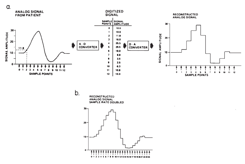
The accuracy with which a computer represents the fine structure, and therefore frequency content, is determined, in part, by the number of sampled points on the waveform (see Figures 1a and 1b). This number depends on the maximum sampling rate of the A-D conversion process, which is inversely related to how long each conversion takes. The amount of time required for the A-D converter and computer to sample each point is called the dwell time. The sampling rate thus determines directly the temporal resolution of the waveform.
Amplitude resolution depends on the numeric precision of the A-D converter, which is specified by the number of bits or places in the binary number representing its full-scale range of sensitivity. For example, suppose a 4-bit A-D converter were used to measure the voltage of a common flashlight battery, and that this A-D converter had a sensitivity of ±5 V. The voltage of a flashlight battery is 1.5 V. Converted from binary to decimal, the numbers that are available to represent the measured voltages fall within the range of 0 to 15 (i.e., from no bits set to all bits set), as shown in Table 1. The actual voltage of the battery does not fall exactly at an integer value, but neither does 0 V. This A-D converter therefore could only approximate the actual binary equivalent of the voltage, and any voltages falling between -0.33 V and +0.33 V would be represented as 0.
| Binary | Decimal | Voltage |
|---|---|---|
| 1111 | 15 | + 5.00 |
| 1110 | 14 | + 4.33 |
| 1101 | 13 | + 3.67 |
| 1100 | 12 | + 3.00 |
| 1011 | 11 | + 2.33 |
| 1010 | 10 | + 1.67 |
| 1001 | 9 | + 1.00 |
| 1000 | 8 | + 0.33 |
| 0111 | 7 | - 0.33 |
| 0110 | 6 | - 1.00 |
| 0101 | 5 | - 1.67 |
| 0100 | 4 | - 2.33 |
| 0011 | 3 | - 3.00 |
| 0010 | 2 | - 3.67 |
| 0001 | 1 | - 4.33 |
| 0000 | 0 | - 5.00 |
Signal averaging is necessary because the AEPs must be extracted from much larger background noise. Poor SNR is overcome by summing numerous digitized wave forms, each timed-locked to the stimulus. Synchronous events that are time-locked to the stimulus should have like phases and thus will summate and “grow” out of the noise background. Any events that are not time-locked to the stimulus (i.e., most of the background noise) will have randomly varying phases (from epoch to epoch) and will tend to cancel out, leaving only the time-locked signal (waveform). The improvement in SNR is proportional to the square root of the number of samples that are summed (averaged) (Picton & Hink, 1974). Thus, increasing the number of samples by a factor of 4 will increase the SNR by a factor of š4 = 2. One of the limiting factors for SNR improvement is the precision of the A-D conversion. Eight-bit resolution appears to be adequate for most evoked potential measurements. Current commercial test instruments employ 8–12-bit converters.
Amplification
The small amplitude of surface-recorded EPs necessitates the use of amplification prior to signal averaging. The objective is not only to amplify the recorded potentials, but also to optimize the voltage sampling for the desired potential while rejecting unwanted signals common to each of the amplifier inputs. This principle is illustrated in Figure 2. The differential amplifier has one input that inverts (-) and one that does not invert (+) the signal at the amplifier's output. The amplified signal is the difference between the two inputs; specifically this signal is the algebraic difference between the two inputs at each instant in time. Any signal common to both inputs therefore is canceled or rejected; this is known as common mode rejection (CMR). Each channel of recording requires one electrode as a ground and two electrodes to pick up the desired potential. All three electrodes generally are placed on the head for EP recordings. Most myogenic artifacts and extraneous electrical noises will appear at the two electrode sites with nearly equal amplitudes and phases because of their proximity and therefore will be rejected. Other signals will not be rejected and, indeed, may be enhanced, as illustrated by Figure 2. Common mode signals may be larger than differential signals, depending on the electrode location relative to the location and orientation of the source of the desired potential. The details of electrode placement will be discussed later within the context of specific test procedures.
Figure 2. Differential amplification. The high-frequency signal is common mode (same amplitude and phase at the two inputs) and is rejected. In contrast, the low-frequency signal is of opposite phase and is enhanced.
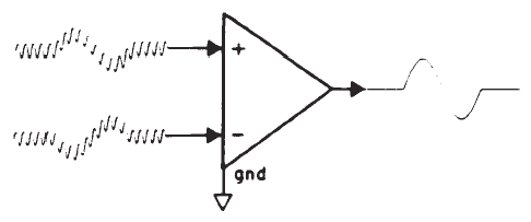
There are several specifications of the amplifier (sometimes referred to as a preamplifier) that are important. One is amount of CMR, which usually is specified in decibels and is defined as the amount of amplitude reduction of common signals. Commercially available bioelectric amplifiers are capable of CMRs of 80–120 dB, which is sufficient for EP measurements. It cannot always be assumed, however, that the amplifier is properly adjusted to permit this amount of CMR, and an occasional check and perhaps readjustment (as per the manufacturer's recommendation) are required. Although CMR is dependent on the balance between electrodes, if electrode impedances are less than 5 kohms, then concerns for balance are reduced because of the high input impedance of differential amplifiers. The input impedance should be a minimum of 1 Mohm, so as not to draw any significant amount of current from the electrodes.
The gain of the amplifier depends on the full-scale voltage range of the A-D converter and minimum voltage input requirements. Typical gain values for evoked response systems range from 10,000 to 500,000. The objective is to present the A-D converter with a signal whose voltage is nearly full scale. For example, if an A-D converter were used with a ± 5 V range (i.e., 10 V full scale) and the recorded signal (including background noise) were 10 µV (0.00001 V) peak to peak, then a gain of approximately 100,000 (i.e., 10/0.00001) would be needed.
All electrical circuits create some thermal noise, and this noise may be amplified. Internal noise should be below 10 µV peak-to-peak to maximize SNR improvement achieved by signal averaging. The amplifier also should be able to withstand the accidental occurrence of relatively high voltages across its inputs, or overvoltaging, and it should be able to recover expediently. A certain amount of mishandling of the amplifier is inevitable in clinical situations. One example is removing the electrodes from the subject before disconnecting them and thereby turning the electrode leads into antennae for electrical noise from the lights and wiring in the test area. The amplifier should be able to take such abuse without electronic failure. Overvoltaging reflects amplifier saturation. Therefore, it is important that overvoltaging not occur during response averaging because this form of nonlinear amplification can affect the signal averaging process. Techniques such as artifact rejection suspend averaging during overvoltaging and the subsequent recovery period. Finally, baseline (dc) drift should be negligible to ensure stability over long test sessions.
All of these specifications are readily met by modern bioelectric amplifiers. However, manufacturers of EP test equipment provide few protocols for checking these parameters and typically do not give amplifier specifications in their manuals.
Filtering
The spectra of most EPs are concentrated such that much of the background noise can be removed via filtering. Filtering can be done before and/or after the signal averaging, but some prefiltering usually is incorporated in the (pre)amplification process, prior to averaging. Filtering must be applied judiciously and with knowledge that it may distort the waveform of the desired potential and may influence latency and amplitude measurements. Analog filtering introduces phase shifts that become increasingly severe as the cutoff frequency of the filter approaches the lower frequency limits of the spectrum of the potential. Not all components of a recorded potential are optimally filtered using the same filter settings and/or response characteristics of the filter. Conversely, not all potentials or components are affected in the same manner by a given filter response. In some recording amplifiers a single-stage (single-pole), passive (resistance-capacitance) filter is used that provides a rejection slope of 6 dB/octave. Others may have two or more stages and/or utilize one of various active filter circuits to provide other response characteristics and/or higher rejection slopes. The cutoff frequency generally is specified at the half-power point of the filter's response, which is the frequency at which the filter's response is 3 dB down from its maximum response.
It is desirable to high-pass filter, or ac couple, to eliminate very low frequency and dc potentials. These potentials cause drift in the baseline of the recording and tend to make the recordings vulnerable to movement artifacts. The front-end differential amplifier is dc coupled, so the filtering or ac coupling is done at a later stage of amplification. Consequently, care must be exercised to minimize the presence of large dc or very low frequency ac potentials at the amplifier's inputs. This can be accomplished by using proper skin preparation, using large-surfaced and reversible electrodes to keep impedances low, and minimizing electrode movement.
Low pass filtering is needed because high frequency noise can be superimposed on the tracing and can obscure peak EP identification. The use of low pass filtering also is determined by the sampling rate of the A-D converter. Consequently, there is an upper frequency limit for the allowable spectrum of the signal being processed. If this frequency is exceeded, there is wraparound or aliasing of the signal's spectrum, in which frequencies above a certain frequency are represented as lower frequencies in a predictable manner. Because there must be at least two sample points to define a cycle of a waveform, the upper limit of permissible frequencies is one-half the sampling rate of the A-D conversion (e.g., 5000 Hz if the sampling rate is 10000 Hz). The highest permissible frequency is called the Nyquist frequency (Nyquist, 1924). For example, a complex tone made up of 3000 Hz and 6000 Hz will appear to be made up of 3000 Hz and 4000 Hz components if the sampling rate is 10000 Hz (Nyquist frequency is 5000 Hz). This occurs because 6000 Hz exceeds the Nyquist frequency and is represented at its aliasing frequency of 4000 Hz (this is the difference between the sampling rate and the true frequency to be analyzed or 10000 Hz minus 6000 Hz). In practice it is necessary to be even more conservative if the actual waveform is to be adequately reproduced, as is the case in evoked response work. An upper limit of less than or equal to one-half the Nyquist frequency or one-fourth the sampling rate (in the above example, -2500 Hz) is more appropriate (Picton & Hink, 1974).
Some high frequency noise is likely to remain, even with low-pass filtering. This may be treated via some form of post filtering or smoothing, which is a form of low pass filtering. Many signal averaging systems provide some type of smoothing function. The most common approach is the sliding average in which each point is averaged with one or more adjacent points. Care must be taken that the smoothing algorithm itself does not cause time delays or that such delays are correctable. In general, digital filtering provides more precise filter skirts and zero phase shift, minimizing the problems associated with analog filtering and certain smoothing algorithms. Although digital filtering has become more widely available, many instruments still utilize a combination of analog filtering and digital smoothing.
Artifact Rejection
Recording a well-defined response depends on the initial SNR, the number of samples averaged, and the extent to which the noise background is truly random. It is possible that an event will occur during averaging that may not be canceled by a clinically practical number of samples. For example, an incidental swallow can create a large electromyogenic artifact that may not be averaged out. Signal averaging can provide substantial noise reduction, even with the occurrence of such incidental fluctuations in the noise background; however, it generally is best to exclude unusually large amplitude noise samples.
Many artifacts encountered in EP recordings are sufficiently large in relation to the desired potential that they can be excluded on the basis of their amplitude. Most commercially available test systems include the capability of specifying an acceptable input amplitude window or adjusting the input sensitivity while testing for samples exceeding full scale. Artifact rejection schemes are most effective in eliminating samples containing incidental voltage spikes but are relatively ineffective in dealing with continuously high levels of noise. Increasing the threshold for artifact rejection or reducing the amplifier gain merely admits more noise without improving the SNR because the SNR is essentially unchanged.
Shielding and Related Issues
The amplification required for the recording of the short latency and other AEPs makes it easy to pick up extraneous electrical noises via electrostatic and/or electromagnetic coupling. The former is exemplified by the reception of 60 Hz noise from a fluorescent light, and the latter is exemplified by reception of 60 Hz noise induced in the amplifier circuit by radiation from a power transformer, electrical machinery, or electrical wiring around the test room. Electromagnetic fields also are created by earphones and similar transducers, and are the most prominent source of stimulus artifact. Precautions to minimize such artifacts include the careful separation of the earphone wires from the electrode wires, draping the electrode leads close to the subject's body, braiding and/or shielding electrode leads, and making the electrode leads as short as practical.
Earphones can be electromagnetically shielded using one or more layers of mu-metal (Elberling & Salomon, 1973), a material that tends to encourage the cancellation of the magnetic field. It also provides electrostatic shielding if it is grounded. The manner in which it is applied, however, may alter the acoustics of the earphone.
A particularly effective way to reduce stimulus artifacts was described by Sohmer and Pratt (1976), in which a tube is used to couple the earphone to the subject's ear and thereby create an acoustic delay line. There has been a growing interest in the use of certain types of insert earphones, which provide the advantage of the delay line effect (e.g., see Clemis, Ballad, & Killion, 1986). There now are commercially available insert earphones with output characteristics similar to the Telephonics TDH-39 earphone. The transducer unit is positioned away from the ear, and the sound is directed through a flexible plastic tube that is coupled to the ear canal with an earplug. The delay imposed by the tube must be taken into account when determining absolute response latencies, in order to obtain values consistent with those obtained with conventional earphones. Latencies obtained with this type of insert earphone will be several tenths of a millisecond or more longer than those observed from responses stimulated via conventional earphones. Insert earphones have the added advantages of increased comfort and more interaural attenuation, reducing the need for masking of the nontest ear.
Interference from 60 Hz noise can be minimized by choosing stimulus rates such that the interstimulus interval equals an odd multiple of one-half the period of 60 Hz (i.e., 8.333 msec). For example, at 17 stimuli per second, the interstimulus interval = 1/17 = 58.8 ms ∼7 x 8.333 ms. Similarly, stimulus artifact can be reduced by presenting stimuli of alternating polarity/phase or randomly varying phases. Some caution must be exercised in applying this method in that, if there is distortion in the stimulus artifact, cancellation will not be complete. Cancellation using alternating phases also can obscure potentials that may be desired. Finally, some commercial instruments provide the possibility of zeroing the initial part of the response tracing in which the artifact is prominent. This can minimize the effects of stimulus artifacts on response scaling but does not eliminate artifacts or their effects on the quality of the recorded responses.
Proper electrical wiring of the sound production and response recording systems is important, not only to minimize electrical artifacts but also to minimize electrical hazards (Pfeiffer, 1974). Evoked response test equipment should be evaluated for electrical safety in accordance with published standards (e.g., Joint Commission on Accreditation of Hospitals, 1987). An EP system should never be used without an intact three-pronged, hospital-grade line plug, nor should it be plugged into an electrical outlet not known to be free of ground faults. The use of a three- to two-prong adapter is unacceptable. The test instrument and outlet to which it is connected should be checked by a qualified electrician or electrical safety officer. The use of faulty equipment, faulty wiring, or improper grounding must be avoided.
Consideration must be given to the location of evoked response testing, both with regard to electrical and acoustical shielding. A metal sound isolation chamber, designed especially for electromagnetic and electrostatic shielding, is ideal but not essential in every situation. The need depends on the electrical and acoustical environment. Because testing is usually done under earphones, a quiet office may prove adequate for some applications (e.g., otoneurologic evaluations involving only high level stimulation).
Outputting Data
The final determinant of the fidelity with which the waveform of the EP is reproduced depends on the manner in which the data are plotted. In the case of digital plotters, wherein the X and Y coordinates are changed in steps, the reproduction will be true to the form of the digitized wave, except that there will always be a slightly jagged character in the detail of the waveform due to the stepping action of the pen (somewhat like the waveform shown in Figure 1b). The smoothness of the tracing will depend on the resolution associated with the analysis, the rate at which the plotter works, and instrument characteristics that are rarely under user control.
The outputting of data via analog devices, such as the X-Y plotter, requires digital-to-analog (D-A) conversion of the data in the computer's memory. Some of the same considerations given to A-D conversions apply to D-A conversion although, in practice, the demands are much less in terms of dwell time and resolution.
Sound Stimulation
Spectrum: Clicks Versus Tone Bursts. Temporally concise stimuli result in synchronized neural discharges and robust EPs. Unfortunately, temporal specificity of the stimulus is achieved at the expense of frequency specificity. A click is a sound obtained by applying a dc pulse to an earphone or loudspeaker (Figure 3a.1), and it provides an excellent stimulus for eliciting the short latency potentials. Its abrupt onset and brief duration contribute to good synchronization, minimize stimulus artifact, and provide a broad spectrum that stimulates many nerve fibers. However, the frequency response of earphones may alter the spectrum of a dc pulse (Figure 3a.2). The auditory system itself also filters the stimulus. Thus, there always are frequency limits imposed on the click-evoked potential (Durrant, 1983).
Figure 3. (a.1) Acoustic output of an earphone (Telephonics TDH-39) in response to direct current pulses applied to the earphone input, producing clicks initiated by condensation (con.) or rarefaction (rar.) phases. (a.2) Spectrum of the acoustic output, that is the click (solid line), versus the electrical pulse (dashed line) driving the earphone. From “Fundamentals of Sound Generation” by J.D. Durrant, in E.J. Moore (Ed.), Basis of auditory brainstem evoked responses (p. 31). New York: Grune & Stratton. Copyright 1983 by Grune & Stratton. Adapted by permission. (b) Spectrum of a brief tone burst, showing main central lobe sidebands.
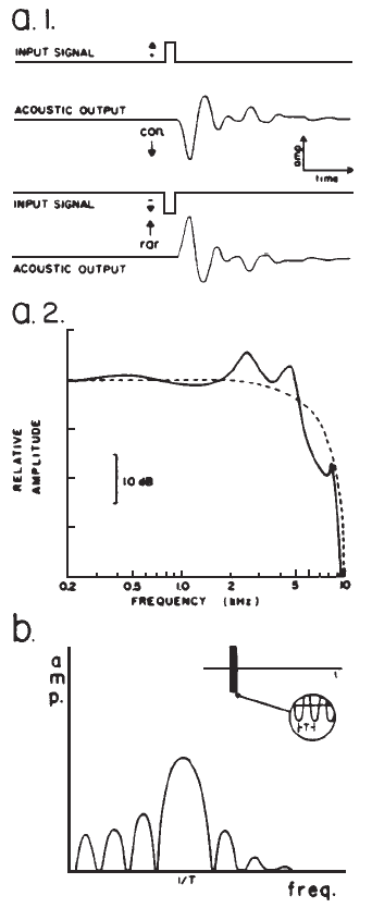
When frequency specificity is desired, sinusoidal pulses (tone pips or bursts) or band-pass filtered clicks may be used. Because such stimuli are transients, their spectra are characterized by energy spread around the nominal or center frequency (Figure 3b). Sinusoidal pulses produce short latency potentials whose latencies vary as a function of frequency (for a given intensity), reflecting somewhat the traveling wave propagation time in the cochlea (Naunton & Zerlin, 1976). Visual detection levels (VDLs) of the auditory nerve and brainstem potentials elicited by filtered clicks and brief tone bursts correlate reasonably well with audiometric thresholds at frequencies at and above 500 Hz. This agreement adds credibility to the assumption that the appropriate frequency region of the cochlea is generating the response.
There are some difficulties with the use of sinusoidal pulses or filtered clicks. First, there may be a broad excitation pattern in the cochlea at high stimulus levels (Bekesy, 1960; Durrant, Gabriel, & Walter, 1981). This is true also for steady state sinusoids, gated sinusoids, and clicks. Second, there is still an intensity dependent latency shift, just as in the case of broadband click stimulation, reflecting the basalward spread of excitation at higher intensities (Folsom, 1984). Third, the shift in latency with frequency reflects, in part, a change in the rise time of the stimulus (e.g., longer at lower frequencies). Fourth, there is a greater chance of contamination from stimulus artifact with these longer stimuli compared to the click. Finally, the amplitudes of short latency EPs diminish and the waveform is less sharply defined as the frequency of the stimulus decreases, especially below 1000 Hz.
Temporal Factors. There are various temporal parameters associated with stimulation, particularly with regard to the use of tone bursts. These include plateau duration, rise/fall duration, and the gating or windowing function by which the amplitude envelope of the sinusoid is shaped (e.g., rectangular, cosine, logon, etc.). The short latency potentials are relatively insensitive to the plateau duration of the stimulus because they are largely onset responses. The rise-fall duration, however, does affect these responses. Generally speaking, the slower the rise time, the lower the amplitude and the longer the latency of the evoked response. The resulting changes in the EPs presumably are the result of decreased synchronization of discharges to stimulus onset, the concomitant decrease in stimulus amplitude near the instant of onset, and the narrower bandwidth of the stimulus as stimulus rise time is increased. The shape of the gating function also influences the stimulus spectrum, and some functions result in greater concentration of energy than others in the main spectral lobe and lower energy in the sidebands (Harris, 1978; Nuttall, 1981).
Stimulus repetition rate is also an important parameter. The repetition rate of the stimulus must be slow enough to prevent significant adaptation of the response. Repetition rates of 10/second or less do not significantly affect the short latency potentials, but rates of 20/second or more are often satisfactory for clinical purposes. Higher rates improve efficiency of data collection but jeopardize the identification of a response or certain component waves of the EP, particularly in some pathological cases. Because there are effects of increasing repetition rate specific to each of the short latency potentials, further discussion will be reserved for later.
Stimulus Calibration. Calibration of the test stimulus is an integral part of evoked response evaluation. The intensity of a click is frequently reported in dBnHL, which is the number of decibels above the behavioral threshold of a group of normal listeners. (Note: this measure has been referred to variably in the literature as nHL, HL, nSL, or SL.) Although the nHL can serve as a useful clinical reference, it does not provide a physical measurement of intensity that permits checks of stimulus output or comparisons across clinics. Calibration procedures are difficult because of the transient nature of the stimuli employed. Sound level meters typically used for audiometric calibration require long duration signals for accurate measurement. Different techniques must be utilized to measure the amplitude of brief stimuli.
Although no standard calibration procedure exists for clicks and other transients, a popular approach is to determine the peak equivalent sound pressure level (peSPL). This measurement is obtained by using an oscilloscope to match the amplitude of a sine wave with the peak amplitude of the click stimulus. The amplitude of the long duration pure tone can then be measured on a sound level meter. Stapells, Picton, and Smith (1982) showed that 0 dBnHL for clicks occurs at approximately 30 dB peSPL. An alternative procedure is to use a sound level meter that can capture transients such as clicks.
Stimulus polarity does not affect the amplitude spectrum (Figure 3a), but it can affect the short latency potentials. Therefore, it is essential to measure the starting phase of the signal to determine whether the stimulus begins with condensation or rarefaction (Figure 3a.1). The phase of the stimulus can be examined by connecting the output of a sound level meter to an oscilloscope and comparing the phase of the stimulus to a known pressure change (Cann & Knott, 1979).
The spectrum of the stimulus should be measured if the instrumentation is available. The temporal features of the stimulus waveform also should be examined. The transient response of an earphone should be characterized by minimal ringing (i.e., minimal overshoots at the onset and offset of the stimulus). The waveform should be scrutinized for changes that may occur over time, especially with an earphone that may have been dropped or otherwise abused. To ensure comparable acoustic stimuli to each ear, the two earphones should create stimuli of nearly identical wave forms. Again, such observations can be made with the aid of a sound level meter coupled to an oscilloscope. If an oscilloscope is not available, then the signal averaging system can be used (Weber, Seitz, & McCutcheon, 1981).
Finally, when determining hearing levels, the psychophysical method for threshold measurement and number and rate of stimulus presentations are important factors. The integrity of the hearing of the normative group sample must be affirmed. All of these factors should be documented and referenced in the hearing level specification until such time that a national standard is developed. For more in-depth discussions of these and other aspects of stimulus calibration (e.g., choice and effect of pulse duration for click stimulation), the reader is referred to chapters by Durrant (1983) and Gorga, Abbas, and Worthington (1985).
Bone Conduction. In conventional audiometry the magnitude of conductive lesions is assessed by comparing thresholds obtained via air versus bone conduction stimuli. It is also possible to use this approach in evaluations of AEPs (although conductive lesions manifest themselves in other ways, as discussed below).
The efforts to date to integrate bone conduction stimulation in testing the short latency potentials have centered around the use of conventional audiometric bone vibrators with AEP test instruments (see Schwartz, Larson, & DeChicchis, 1985). Unfortunately, even when the earphone and bone vibrator outputs are adjusted for equal sensation levels (for clicks), the bone conduction elicited response is delayed by 0.5 ms or more (Weber, 1983). Some investigators have attributed this delay to the poor high frequency response of the bone vibrator (Mauldin & Jerger, 1979). The bone vibrator tends to have a major spectral peak between 1 and 2 kHz with a substantial roll-off in the frequency response above about 1.6–2.5 kHz. Therefore, air and bone conduction clicks have different spectra. This has been revealed by comparing the earphone output measured in a 6 cm3 cavity with the bone vibrator output measured on an artificial mastoid, as well as measures rendered in terms of estimated hearing levels (Schwartz et al., 1985).
The output of the vibrator is around 40 dB below that of the earphones, even when both are driven to saturating levels of output, just as in the case of pure tone audiometry. However, the realizable hearing levels (i.e., 40–50 dB) permit only relatively mild conductive hearing losses to be quantified. Thus, the absence of a click-evoked potential by bone conduction does not necessarily imply solely sensorineural impairment; a moderate or more severe degree of mixed loss might be involved. Conversely, due to the low frequency emphasis of the bone conduction click, a conductive lesion could be erroneously deduced when, in fact, there is a precipitously sloping high frequency loss. However, this problem can be vitiated with the use of tympanometry, acoustic reflexes, and the measurement of Wave I latency.
There is one other problem with existing bone vibrators. Like the conventional earphone, the bone vibrator is an electromagnetic device and therefore emits electromagnetic waves, causing stimulus artifact. The bone vibrator is actually a worse offender due to its lower efficiency (i.e., a higher voltage driving signal is necessary to obtain the same hearing level as that obtained using an earphone).
Despite these limitations, most evoked response audiometer manufacturers now offer bone conduction options, and support has been expressed for the use of bone conduction in AEP testing (Berlin, Gondra, & Casey, 1978; Mauldin & Jerger, 1979; Weber, 1983). Bone conduction testing can help in newborn screenings and other audiologic applications but, clearly, care must be taken in the use and the interpretation of results obtained.
Electrocochleography
Electrocochleography (ECochG) is a term that has been applied to a family of electrophysiologic techniques directed specifically toward the recording of stimulus related potentials generated from the cochlea and eighth nerve. Attempts at clinical applications of ECochG date back almost as far as the discovery of the cochlear potentials by Wever and Bray (1930), but practical applications were not realized until the late 1960s. However, work in this area decreased over the next decade as the clinical interest in ABRs expanded. Recently, there has been renewed interest in ECochG in assessing and monitoring certain audiologic/otologic and neurologic disorders, in monitoring surgical procedures, and in supplementing ABR measurements (Ferraro, 1986).
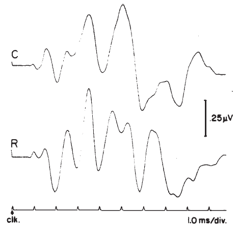
The record of the potentials recorded via ECochG is called the electrocochleogram (ECochGm). Although the ECochGm consists of more than one electrical potential (Figure 4), the most obvious and most easily recorded component is the whole nerve action potential (AP) of the eighth nerve. The AP is characterized by a series of one to three predominantly negative waves, the largest of which is known as N1 (Figure 4). The AP N1 component is the most salient feature of the ECochGm (Coats, 1974).
Figure 4. Component potentials of the (human) electrocochleogram recorded from the ear canal using condensation (C) and rarefaction (R) click stimuli: N1, major component of the whole-nerve action potential (AP); CM, cochlear microphonic; SP, summating potential. The CM and SP can be selectively enhanced by manipulating the R and C responses, as indicated. Ear-canal negative (-EC) potentials are plotted as downward deflections. (Based on data from Coats, 1981.)
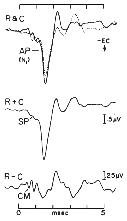
The stimulus related potentials generated by the hair cells (i.e., prior to excitation of the auditory nerve) are the cochlear microphonic (CM) and the summating potential (SP). The CM has a similar waveform to the stimulus. For example. if a tone burst is presented, a sinusoidal voltage is recorded. The recorded potential, however, often is asymmetrical, with its zero axis offset from the baseline. This is due to the presence of the SP. The SP can be isolated via low-pass filtering or phase cancellation of the CM (Figure 4). Depending on the combination of stimulus parameters and recording site and method, the SP may be of either positive or negative polarity. When elicited by a transient stimulus such as a click, the SP appears as a transient deflection on which the AP is superimposed and forms a shoulder on the leading edge of the AP waveform, as shown in Figure 4 (Coats, 1981). For a more extensive treatment of these potentials, the reader is referred to Dallos (1973) and to Durrant and Lovrinic (1984).
Recording Techniques: Electrode Type and Montage
There are two general recording techniques available for ECochG. One method involves inserting a needle electrode through the tympanic membrane (TM) to rest on the cochlear promontory. The invasive nature of this approach has limited its applications in the United States. Because of this, the use of transtympanic ECochG will not be considered directly in this discussion. (Extra)tympanic techniques utilize recording electrodes located on the lateral surface of the TM or in the ear canal. Cullen, Ellis, Berlin, and Lousteau (1972) first described an extratympanic, surface recording method using a silver ball electrode wrapped in a saline-soaked cotton pledget and placed against the TM. This technique provided good results with minimal discomfort to the subject, although the subject was required to lie down, and the stimulus had to be presented via sound field. A recently designed extratympanic electrode (Stypulkowski & Staller, 1987) has rekindled interest in this approach to ECochG as it largely obviates problems with older designs.
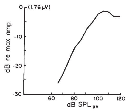
Coats (1974) introduced an electrode assembly that is self-retaining, although the point of recording was moved away from the eardrum and onto the floor of the ear canal. This electrode is illustrated in Figure 5. A light, flexible but springy clip is used to hold a silver ball electrode against the canal wall. This electrode can be used under earphones, provides good recordings, and visual detection levels (VDLs) in many subjects approximate the behavioral threshold of the stimulus (see Figure 6).
Figure 5. An electrode assembly for recording from the ear canal: (A) silver ball electrode supported by retainer made of acetate; (B) assembly held by forceps as required for insertion; (C) placement in the ear canal. From On Electrocochleographic Electrode Design by A.C. Coats, 1974, Journal of the Acoustical Society of America, 56, p. 79. Copyright 1974 by the American Institute of Physics. Reprinted by permission.
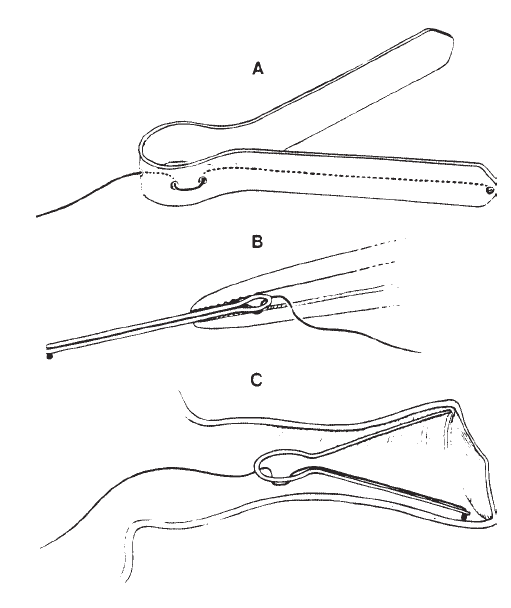
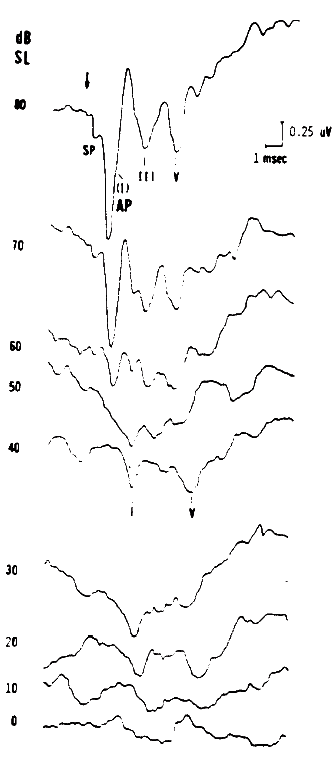
Figure 6. Combined electrocochleogram and brainstem potential recording at different sensation levels of the click stimulus. Recording montage: ear-canal electrode connected to the noninverting input of the differential amplifier, surface electrode placed on the forehead at midhairline connected to the inverting input; surfacer electrode over the zygomatic process connected to ground. By virtue of this recording montage, both ear-canal negative potentials and forehead/vertex positive potentials are plotted as downward deflections. From Combined ECochG-ABR Versus Conventional ABR Recordings by J.D. Durrant, 1986, Seminars in Hearing (Electrocochleography), 7, p. 292. Copyright 1986 by Thieme Medical Publishers. Reprinted by permission.
Inherent problems with this type of ear canal electrode are the difficulty of controlling placement and the relatively high electrode impedances. Impedances typically are in excess of 20 kohms (Durrant, 1986). With modern preamplifiers and their very high input impedances, the magnitude of the electrode impedance is not as much of concern as is the balance between each branch of the circuit formed in connecting the differential amplifier to the patient. The balance between electrode pairs is generally poor, and this degrades CMR and noise suppression. Higher impedances also create more noise artifact.
Other ear canal electrode designs have been described that are placed closer to the entrance to the ear canal (e.g., Whitaker & Lewis, 1984; Yanz & Dodds, 1985). Also, an earplug electrode of this general type compares favorably with the Coats electrode, when the latter is inserted near the entrance to the ear canal (Ferraro, Murphy, & Ruth, 1986). These more recent designs have substantially reduced the impedance problem due to their effectively large surface areas. The amplitude of the recorded potential, however, is reduced for less deep electrode placements (Coats, 1974). These electrodes do appear to provide useful recordings of the AP and the SP. The earplug electrode assembly is similar to tubal insert earphones. Thus, the response is much less susceptible to stimulus artifact, compared to responses obtained with other types of ear canal electrodes used in conjunction with the conventional earphone.
It will be recalled that in differential recordings a second electrode, sometimes called the reference electrode, is required, along with a ground electrode. Two possible placements for the reference electrode are the ipsilateral earlobe and mastoid. Some of the desired potential, however, will be canceled by the differential amplifier because neither the ipsilateral earlobe nor the ipsilateral mastoid is totally inactive. Preferable sites for the reference electrode are the nasion (just above the bridge of the nose) or contralateral earlobe/mastoid, which are relatively inactive for the ECochGm. Durrant (1977, 1986) also suggested recording between the ear canal and the vertex or forehead to provide simultaneous pickup of the eighth nerve and brainstem components, as illustrated by Figure 6. Although this works well in some cases, in other cases the AP may not be picked up much better in the ear canal than on the earlobe or mastoid and in still others the AP can be overwhelmingly large (thereby interfering with the resolution of the brainstem components). Nevertheless, this approach may help to enhance the eighth nerve component (Wave I) of the ABR (Durrant, 1986; Eggermont, Don, & Brackmann, 1980). Alternatively, a two-channel system can be used to record simultaneously from ear canal and surface electrodes and thus separately monitor eighth nerve and brainstem responses (Coats & Martin, 1977).
Another form of noninvasive ECochG is that of recording via a scalp/surface electrode placed on the earlobe or mastoid. Even prior to the appearance of the classic paper by Jewett, Romano, and Williston (1970) describing ABRs, Sohmer and Feinmesser (1967) described ECochG using essentially the same electrode placements. The differences between these studies were the polarity reference and the presumed sources of the responses. Jewett and his associates considered the vertex to be active, and Sohmer and Feinmesser considered the earlobe to be active. Both are really active, but the earlobe (or mastoid) is more active for the AP, and the vertex is more active for the brainstem components. Indeed, it is well established that the ECochGm forms the initial part of the ABR as illustrated by Figure 6.
Comparisons among tympanic membrane (TM), ear canal, and surface ECochG recordings have recently appeared in the literature (Ferraro & Ferguson, in press; Ferraro et al, 1986; Stypulkowski & Staller, 1987; Ruth, Lambert, & Ferraro, in press; Ruth, Mills, & Ferraro, in press). As expected, recordings from the TM yield the largest, most sensitive and reliable responses among the three approaches. Although it is possible to record the AP or even the CM (Sohmer & Pratt, 1976) from the earlobe or mastoid, recordings from these sites suffer from substantial reduction in sensitivity compared to ear canal recording techniques (Ferraro et al., 1986). Reliable recordings of the SP from sites as remote as the earlobe/mastoid have yet to be demonstrated.
Stimulus Variables
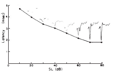
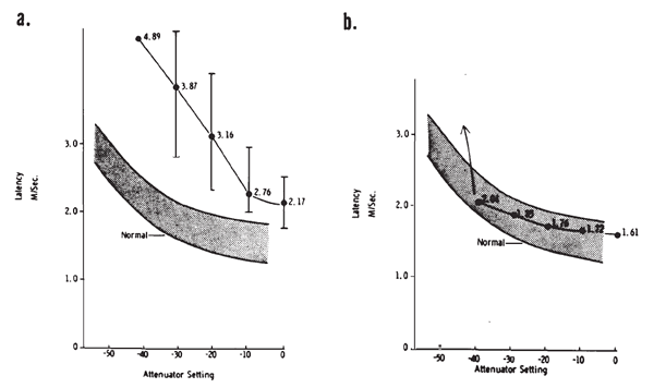
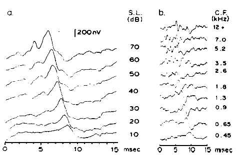
Intensity. Compound APs grow in proportion to the amplitude of the stimulus, as shown in Figure 7. AP latency also depends on the intensity of the stimulus. The latency of the AP is defined as the delay between the onset of the stimulus and the occurrence of the N1 response peak. The graph of latency versus stimulus level is called the latency-intensity function (Figure 7). These data demonstrate that as the stimulus intensity decreases, latency systematically increases.
Figure 7. AP latency-intensity function and corresponding ECochG tracings (recorded via an ear-canal electrode).
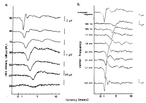
The latency-intensity shift of the AP is demonstrated further by the ECochGm shown in Figure 8a. The basis of this phenomenon is evident from the recordings presented in Figure 8b. The latter ECochGms were obtained in the presence of different high pass noise maskers. The subtraction of the response obtained with a masker of lower frequency cutoff from that obtained with a masker of higher frequency cutoff yields the contribution largely of neurons innervating the cochlear region between the places marked by the cutoff frequencies (Teas, Eldridge, & Davis, 1962). The high level response is dominated primarily by the contributions of fibers located near the base (high frequency region) of the cochlea, whereas the contributions from lower frequency regions tend to cancel one another (Eggermont, 1976a). The low level responses shown in Figure 8a have latencies corresponding to responses generated by bands centered around 2000 Hz, which is consistent with the greater sensitivity of the 2000 Hz region near threshold. The latency-intensity shift, therefore, is primarily a reflection of the time required for the traveling wave to propagate to the corresponding place along the basilar membrane. As discussed earlier, the click has a broad spectrum but the same mechanism is involved even with more frequency specific stimuli such as tone bursts. Because more basalward fibers will be recruited as the level of the stimulus is increased, the latencies become shorter. The important point is that different populations of neurons dominate the AP at different levels and frequencies of stimulation.
Figure 8. (a) Wide-band click-evoked APs. From Electrocochleography by J.J. Eggermont, 1976, in W.D. Keidel and W.D. Neff (Eds.) Handbook of sensory physiology, vol. 3: Auditory system: clinical and special topics (p. 650). Berlin, Springer-Verlag. Copyright 1976 by Springer-Verlag, Berlin-Heidelberg-New York. Adapted by permission. (b) Derived narrow-band responses with click stimulus presented at 90 dB peSPL. From Analysis of Compound Action Potential Responses to Tone Bursts in the Human and Guinea Pig Cochlea by J.J. Eggermont, 1976, Journal of the Acoustical Society of America, 60, p. 1135. Copyrighted 1976 by the American Institute of Physics. Adapted by permission. Both sets of recordings are from the promontory via a transtympanic electrode.
Both the CM and SP have very short latencies and no significant dependence of latency on intensity of stimulation. The CM magnitude, if represented in logarithmic units, grows in direct proportion to sound pressure in decibels, usually with a slope of unity. As shown in Figure 9, its output saturates at high levels of stimulation and even decreases with continued increases in intensity (Dallos, 1973).
Figure 9. CM input-output function (based on mean data from a sample of normal hearing subjects). Stimulus was a 1-kHz tone burst of 5 ms duration; recordings from needle electrode in the floor of the ear canal, proximal to the ear drum. (Figure modified and redrawn from Elberling & Solomon, 1973.)
The behavior of the SP is more complex overall than that of the CM (Dallos, 1973). Generally, only a negative SP is seen in normal hearing human subjects (Eggermont, 1976b). The SP input-output function from transtympanic recordings is characterized by approximately proportionate growth with stimulus intensity, similar to the CM (when the input-output function is plotted in log-log coordinates) but without much evidence of saturation.
Spectral and/or Temporal Variables. The effects of stimulus spectrum and/or temporal characteristics on the short latency potentials were discussed in general terms earlier, but there are some matters of specific interest with regard to the elicitation of the ECochGm. One relevant variable is stimulus phase. As illustrated by Figure 4, the CM is phase sensitive, whereas the SP is not, and the AP is only slightly phase sensitive (Coats, 1981). Also, the use of tone bursts that typically outlast the click requires particular care in ECochG because of possible contamination from electromagnetic radiation from the earphone. Again, acoustic delays or electromagnetic shielding can be used to minimize stimulus artifacts.
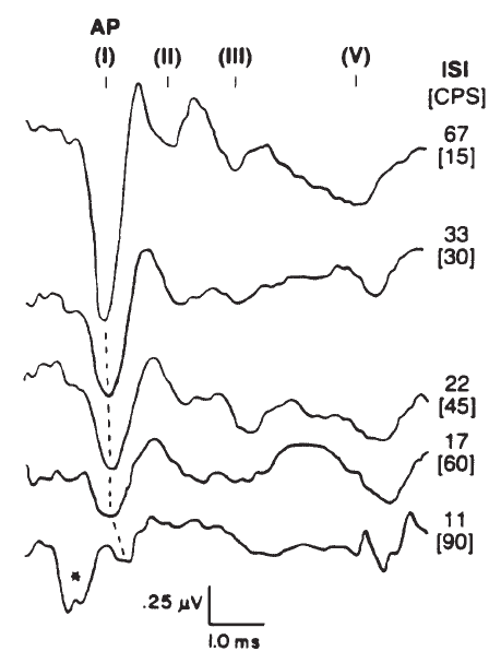
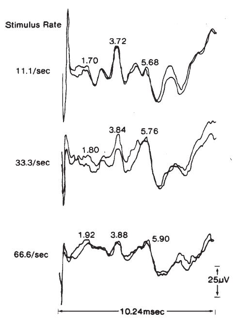
Stimulus repetition rate is an important factor in recording the ECochGm, particularly the AP. As illustrated by Figure 10, the amplitude of the AP decreases and latency increases with increasing rate. In contrast, the SP and CM (although not evident in Figure 10) do not seem to exhibit temporal interactions of any consequence and maintain essentially constant amplitudes regardless of repetition rate. Indeed, one technique employed by some to emphasize the SP is to increase the repetition rate until the AP is maximally depressed (Coats, 1981; Gibson, Moffat, & Ramsden, 1977). This method requires repetition rates on the order of 100/second, but even at such high repetition rates the AP contribution to the recorded response will not be entirely eliminated because the effect of increasing repetition rate is not one of pure adaptation (Durrant, 1986; Harris & Dallos, 1979). The repetition of the stimulus itself causes a certain amount of synchronization of neural discharges, which can occur even at frequencies of several hundred hertz. Otherwise, the AP would completely adapt, rather than accommodating to the repetitious stimulus.
Figure 10. Effects of stimulus rate in clicks per second (CPS); for reference, the interstimulus intervals (ISI) have been computed for each rate tested (*, artifact). The click stimulus was presented at 80 dB SL. AP as well as brainstem potentials (I–V) were recorded via electrodes placed in the ear canal and at vertex. From Combined ECochG-ABR Versus Conventional ABR Recordings by J.D. Durrant, 1986, Seminars in Hearing (Electrocochleography), p. 300. Copyright 1986 by Thieme Medical Publishers. Adapted by permission.
Masking. Fundamentally, the problem of selectively testing one ear is the same for ECochG as it is for conventional audiometry. The problem, however, is far less acute in ECochG, and masking is not used routinely. Masking is unnecessary for most applications of ECochG for two reasons. First, the component potentials of the ECochGm are recorded in a quasi near-field manner (Davis, 1976); consequently, the ECochGm is strongest in the vicinity of electrodes nearest to generators of the cochlear and eighth nerve potentials. Recording on the side of the head opposite the ear stimulated thus yields a substantially attenuated response. Second, due to the substantial transcranial attenuation of sound, the amplitude of a response elicited by crossover stimulation will be greatly reduced, with a concomitant latency shift, compared to that obtained with direct stimulation of that ear.
Subject Variables
Normal Variability. Considerable variability in the amplitude of the ECochGm is typically observed. Even with transtympanic recordings, in which the recorded signal is usually an order of magnitude higher than that obtained via extratympanic methods, AP amplitudes vary by as much as 20:1 (see data of Eggermont, 1976b). Although the extratympanic ECochGm is inherently vulnerable to variance in electrode placement, its variance actually does not appear to be greater than that experienced with the transtympanic method and is comparable to that obtained with surface recordings from the mastoid (Durrant, 1986). The main difficulty with extratympanic methods is a poor SNR that is a result of a reduction in signal amplitude without changes in noise amplitude. Naturally, the more remote the site of recording, the poorer is the SNR.
The variability of latency is much less than that of amplitude and is relatively independent of recording technique. Standard deviations are typically less than 0.2 ms for the AP recorded from normal hearing subjects (Durrant, 1986).
Age and Gender. The effects of age and gender on ECochG have not been studied extensively. Gender differences appear to arise at levels of the system beyond the eighth nerve (McClelland & McCrae, 1979). The only known effects of age are during early development (Fria & Doyle, 1984; Starr, Amlie, Martin & Sanders, 1977). In newborns, particularly premature infants, there is a slight delay in the AP that progressively decreases with maturity. This decrease may reflect maturation of the peripheral system and/or resolution of conductive hearing loss that may be associated with the presence of fluid in the neonatal ear.
Clinical Applications of Electrocochleography
Clinically, AEPs have been used in otoneurologic diagnoses and hearing threshold predictions. ECochG has been used in both of these areas, although the early work involved primarily transtympanic measurements. The discussion here will focus on the clinical utility of extratympanic methods.
Hearing Threshold Prediction. Ear canal ECochG has not proven particularly useful for threshold estimation and does not provide as reliable determinations of threshold estimates as the transtympanic technique (Probst, 1983). It is difficult to record the AP reliably below about 30 dB relative to the individual's behavioral threshold (Cullen et al., 1972). These findings concur with data reported for the early components of the ABR. For some purposes, the gap between AP threshold and behavioral threshold might be acceptable, but the ABR can be recorded reliably near the behavioral threshold and thus has replaced extratympanic ECochG for threshold estimation.
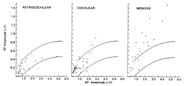
Otoneurologic Applications. The clinical utilities in the area of otoneurologic or differential diagnoses also have been limited for ECochG. Sohmer and his colleagues have applied the surface technique in a variety of cases (Sohmer & Feinmesser, 1973, 1974; Sohmer, Feinmesser, & Bauberger-Tell, 1972). Currently, the most popular clinical application of ECochG is in the identification, assessment, and monitoring of Meniere's disease or endolymphatic hydrops. The primary impetus for this was the work of Coats (1981), following the observations of Eggermont (1976b) and Gibson et al. (1977) that the SP amplitude is altered in many cases. Although the rationale for this finding has yet to be fully explained, it is well documented that the ECochGm of many Meniere's patients is characterized by an enlarged SP, especially in comparison to the AP component (Coats, 1981, 1986; Eggermont, 1976b; Ferraro, Arenberg, & Hassanein, 1985; Gibson et al., 1977; Staller, 1986). This finding is illustrated in Figure 11, which demonstrates the relation between the SP and AP amplitudes for groups of subjects presenting with retrocochlear impairment, cochlear impairment, and Meniere's disease.
Figure 11. Scatterplots of SP versus AP amplitudes for three groups of pathologic ears. The curves represent best-fit estimates of ± 2 standard deviations for responses obtained from normal ears. Recordings from ear canal. From The Summating Potential and Meniere's Disease by A.C. Coats, 1981, Archives of Otolaryngology, 107, p. 205. Copyright 1981 by the American Medical Association. Reprinted by permission.
Originally, it had been hoped that the ECochGm waveform, as well as the input-output and latency-intensity functions, would conform to distinct patterns in cases of different pathologies of the auditory system. As summarized in Figure 12, this goal was partially realized utilizing the transtympanic method (e.g., Aran, 1978). Here it can be seen that cochlear, conductive, and normal patterns are fairly distinguishable. To some extent, similar patterns have been demonstrated using noninvasive techniques as well (e.g., Berlin & Gondra, 1976). Some exemplary latency-intensity data are shown in Figure 13. However, the frequent inability to track the AP down to low levels of stimulation limits the extent to which either the latency-intensity function or the input-output amplitude function can be described. Also, the residual noise in the noninvasive recordings generally precludes accurate typing of the ECochG waveform. These factors have reduced the clinical value of noninvasive ECochG, although it appears that many of them can be overcome by recording from the TM (Stypulkowski & Staller, 1987).
Figure 12. (a) Typical input-output and latency-intensity functions for subjects with normal hearing (A) and conductive (B), recruiting high-frequency (C), and recruiting flat (D) hearing loss. (b) Corresponding ECochG wave forms (transtympanic recordings). From “Contributions of Electrocochleography to Diagnosis in Infancy. An 8-Year Survey” by J.M. Aran, 1978, in S.E. Gerber & G.T. Mencher (Eds.), Early diagnosis of hearing loss, p. 218–219. New York: Grune & Stratton. Copyright 1978 by Grune & Stratton. Adapted by permission.
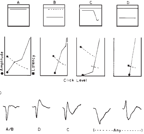
Figure 13. AP latency-intensity functions for group of patients with mild-to-moderate conductive (a) and sloping sensorineural hearing loss (b). Measurements made from recordings from the surface of the eardrum. From Clinical Application of Recording Human VIIIth Nerve Action Potentials From the Tympanic Membrane by C.I. Berlin, J.K. Cullen, M.S. Ellis, R.J. Lousteau, W.M. Warbrough, and G.D. Lyons, 1974, Transactions of the American Academy of Ophthalmology and Otolaryngology, 78, p. 404–406. Copyright 1974 by C.V. Mosby Company. Adapted by permission.
Finally, perhaps the most neglected area of ECochG is the use of the CM. One discouraging aspect is the considerable difficulty of eliminating stimulus artifact to a degree that one is confident that only CM is being recorded. Sohmer and Pratt's (1976) sound delivery system, discussed earlier, was designed specifically for circumventing this problem; they have described successful recordings of the CM using surface electrodes. Despite the support given by some authorities (e.g., Beagley, 1974; Hoke & Lutkenhoner, 1981), the value of CM measurement as a clinical tool has yet to be established.
Measurement of Auditory Brainstem Evoked Potentials
The ABR consists of a series of 5–7 waves, as illustrated in Figure 14. Two labeling systems have been used, one attributable to Sohmer, Feinmesser, and Szabo (1974) and the other to Jewett and Williston (1971), with the latter scheme now being used more widely. The potentials comprising the ABR arise from the auditory nerve, as well as brainstem structures (Jewett, 1970). The simplest view of the genesis of the ABR is that each wave arises from a single anatomical site. However, this view overlooks the complexity of the neural pathways, including bilateral representation, decussation of nerve fibers at various levels, pathways that do not involve synapses at every nucleus, neurons with multiple synapses within a structure, and secondary and tertiary firings of neurons. In humans, Wave II is now believed to arise from the central end of the eighth nerve (Moller & Jannetta, 1982). Only waves beyond II are now believed to represent brainstem level activity. Waves I and II arise from structures ipsilateral to the side of stimulation. Later waves may come from structures that receive ipsilateral, contralateral, or bilateral inputs from the auditory periphery (Achor & Starr, 1980a, 1980b; Buchwald & Huang, 1975; Moller, Jannetta, Bennett, & Moller, 1981; Wada & Starr, 1983a, 1983b, 1983c).
Figure 14. Auditory brainstem response—Jewett Waves I–VII. Onset of click (clk.) stimulus as indicated. Recording montage: surface electrodes at vertex (connected to the noninverting input of the recording amplifier), mastoid (inverting input), and nasion (ground); therefore, following the most widely adopted convention, vertex-positive (+ Cz) potentials are plotted as upward deflections. Peak identifiers in parentheses: terminology from Sohmer and Feinmesser (1967) who used the earlobe for the noninverting input and the bridge of the nose for the inverting input.
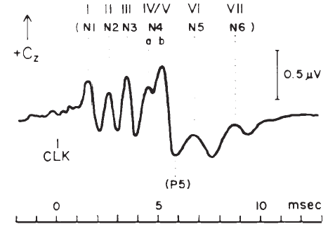
Because Wave I represents the initial response of the auditory nervous system, the later waves tend to mimic its behavior, especially its dependence on stimulus parameters and the status of the middle and inner ears (Davis, 1976). Nevertheless, there is some degree of independence between the brainstem and peripheral nerve components.
Basic ABR Measures
The two parameters of the ABR waveform that usually are measured are amplitude and latency. Amplitude typically is measured between a positive peak and the following negative “peak” or trough (Figure 15). Peak-to-peak measures are favored because they avoid the difficulty of determining the baseline of the potential.
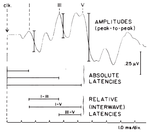
There are several latency measures of interest. The most basic is absolute latency, which is defined as the time difference between stimulus onset and the peak of the wave (Figure 15). Interwave latencies (or interpeak intervals) are the differences between absolute latencies of two peaks, such as I–V, I–III, and III–V (Figure 15). In evaluating ABR latencies, emphasis usually is placed on the vertex-positive peaks of the waveform.
Stimulus Parameters
Intensity. Latency-intensity functions for major components of the click-evoked ABR are shown in Figure 16. The latencies increase as stimulus intensity decreases, roughly in parallel with latency changes in the AP (Wave I). The amplitudes of the waves decrease as the intensity decreases. In addition, as intensity decreases the waves prior to Wave V diminish and ultimately vanish, whereas Wave V often remains discernible down to levels approximating the behavioral thresholds for the same stimulus.
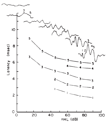
The primary basis for the latency-intensity shift described above is revealed by data from Don and Eggermont (1978), who used the subtractive masking method. This method was developed originally to indicate the regions of the cochlea that contribute to the click-evoked AP (Teas et al., 1962). As shown in Figure 17, different high pass noises are used to obtain masked click-evoked ABRs. The ABR obtained with a lower masker frequency cutoff is subtracted from the response obtained with a higher masker frequency cutoff. The high level unmasked response is dominated by contributions from fibers at the basal end of the cochlea. The latency-intensity shift then appears to reflect the time required for the wave to propagate to the place on the basilar membrane dominating the response. However, if one assumes that this technique results in the masking of basal cochlear regions, then upward spread of excitation cannot entirely account for changes in latency for individual derived bands (see Figure 6 of Eggermont & Don, 1980).
Figure 17. (a) Broad-band click-elicited ABRs. (b) Derived narrow-band responses. From Analysis of the Click-Evoked Brainstem Potentials in Man Using High-Pass Noise Masking by M. Don and J.J. Eggermont, 1978, Journal of the Acoustical Society of America, 63, p. 1087. Copyright 1978 by the American Institute of Physics. Adapted by permission.
Spectrum: Clicks Versus Tone Pips. Clicks are the most commonly used stimuli for eliciting the ABR. The abrupt onset and broad spectrum of a click result in synchronous excitation of a broad population of neurons. The click is usually the most effective stimulus and can provide high frequency information (Coats & Martin, 1977; Don, Eggermont, & Brackmann, 1979; Gorga, Worthington, Reiland, Beauchaine & Goldgar, 1985; Jerger & Mauldin, 1978; Moller & Blegvad, 1976). Tone pips, filtered clicks, or the subtractive masking (derived band) technique must be used for more frequency specific information (Stapells, Picton, Perez-Abalo, Read, & Smith, 1985).
The same concerns that are evident for the use of frequency specific stimuli to elicit the AP are present also for the ABR. Tone pips are transient stimuli, so there is a spread of energy around the central frequency. Second, with increasing intensity the basal fibers progressively dominate the response, regardless of stimulus frequency (Folsom, 1984). This problem exists for conventional pure tone audiometry as well. Third, the effective rise time may become progressively longer as the frequency decreases. This may reduce synchrony in the apical end of the cochlea, making it more difficult to measure. However, the ABR can be elicited with stimuli as low as 500 Hz with appropriate filter settings and sampling epochs (Stapells & Picton, 1981; Suzuki, Hirai, & Horiuchi, 1977). Good agreement has been reported between tone burst ABR and behavioral thresholds at corresponding audiometric frequencies (Suzuki & Yamane, 1982).
The spectrum of the stimulus is influenced by the stimulus plateau and rise/fall durations, as well as by the gating function by which the sound is turned on and off. The brainstem components, like the AP, are relatively insensitive to the stimulus duration (Gorga, Beauchaine, Reiland, Worthington, & Javel, 1984) but quite dependent on the rise/fall times (Kodera, Marsh, Suzuki, & Suzuki, 1983). Response amplitudes decrease and latencies increase as rise time increases. Wave V is the least affected in terms of amplitude decrements with increasing stimulus rise/fall times (Hecox, Squires, & Galambos, 1976).
Various gating functions can be used to minimize spectral splatter of tone bursts (Harris, 1978; Nuttall, 1981). Another approach is to use either notch-band (or stop-band) noise to mask all but the frequency region of the main spectral lobe of the stimulus (Picton, Ouellette, Hamel, & Smith, 1979; Stapells et al., 1985) or the subtractive masking paradigm. The VDL of the ABR can then be determined for each frequency band of interest. These methods may be more technically demanding and time consuming than the use of unmasked tone bursts or filtered clicks.
Polarity. Polarity or starting phase of the stimulus can affect the latencies of the waves and the detailed morphology of the ABR waveform. Different polarities/phases may differentially affect the amplitudes, latencies, and/or resolution of some peaks (Figure 18). For example, the rarefaction phase may elicit ABRs with slightly shorter latencies and better resolution of the peaks in the IVN complex. However, some subjects may show the opposite trends or no significant differences between polarities. When polarity effects are observed, they rarely amount to more than a 0.1–0.2 ms difference in latency in normal hearing, neurologically intact subjects, but the presence of a sloping high frequency hearing loss can cause more dramatic effects (Coats & Martin, 1977). Phase effects seem to depend on the low frequency content of the stimulus (Moller, 1986), although Salt and Thornton (1983) reach slightly different conclusions regarding the sources of the phase effects.
Figure 18. Effects of click polarity (i.e., starting phase) on the ABR: C = condensation; R = rarefaction. From Reconstruction of the Audiogram Using Brainstem Responses and High-Pass Noise Masking by M. Don, J.J. Eggermont, and D.E. Brackman, 1979. Annals of Otology, Rhinology, and Laryngology, 88 (Suppl. 57), p. 6. Copyright 1979 by Annals Publishing Company. Reprinted by permission.
Phase effects are not very great in most subjects. As a consequence, many examiners prefer to use stimuli of alternating polarity, which help to minimize stimulus artifact and the CM, both of which can obscure Wave I. This approach can reduce or eliminate the need for electromagnetic shielding of the earphone. Still, it is generally preferable to keep the phases separate to avoid distorting the ABR waveform. This is particularly important in subjects who have substantially different responses to rarefaction and condensation stimuli. If necessary, the alternating condition can be derived by combining responses for each stimulus polarity in the computer's memory. No information is lost because rarefaction, condensation, and combined responses each can be examined.
Repetition Rate of Stimuli
The amplitudes and latencies of the ABR components are dependent on stimulus repetition rate (see Picton, Stapells, & Campbell, 1981, for a review). As the stimulus rate is increased, the latencies of all the waves are prolonged and the amplitudes of the early waves are decreased. Rates of 10/second or less are necessary for maximal definition of all the waves; the interstimulus interval at this rate is sufficiently long to prevent any significant adaptation of the response for high level stimuli. There is no evidence to suggest that high rates adversely affect the response for low level stimuli. As illustrated in Figure 19, faster rates prolong the latencies of all the waves progressively, so that Wave I is delayed approximately 0.1 ms and Wave V is delayed approximately 0.3 ms between rates of 10 and 50/second (Fowler & Noffsinger, 1983). High rates also decrease the amplitudes of waves prior to Wave V. Waves II and IV are affected the most, followed by Waves I and III. Although rates of 10/second have been proposed to enhance differential diagnoses based on the ABR exam, research findings are not conclusive (Campbell & Abbas, 1987; Fowler & Noffsinger, 1983). Low rates are advisable when a full complement of waves is necessary, such as in the case of otoneurologic evaluations. For other purposes, such as threshold testing, rates of 25–40/second are acceptable because the amplitude of Wave V is minimally reduced. This improves the efficiency of ABR measurements because more averages can be taken in the same period of time.
Masking
There is considerable debate as to whether masking is ever needed. First, at least for clicks, there appears to be greater transcranial attenuation than encountered in pure-tone audiometry (Finitzo-Hieber, Hecox, & Cone, 1979). Further, additional transcranial attenuation can be realized through the use of insert earphones (Clemis et al., 1986). Second, in terms of determining the possibility of retrocochlear pathology, a response to crossover stimuli would be so delayed as to raise as much suspicion as an absent response.
In the audiologic-oriented (sensitivity) evaluation, however, similar considerations for masking must be given as in behavioral audiometry. Contralateral masking is required whenever the stimuli are sufficiently intense as to produce crossover responses. A crossover response will be of smaller amplitude and longer latency, compared to an ipsilateral response, due to the much lower intensity of the stimulus reaching the contralateral ear. Ideally, each clinic should determine effective masking levels for its own equipment and stimuli. The appropriate amount of masking is determined by increasing the level of masking in the nontest ear until the crossover response is eliminated.
Monaural Versus Binaural Stimulation
Binaurally stimulated brainstem responses are larger than monaurally elicited responses by almost twofold (Dobie & Norton, 1980). Binaural stimulation can be used for screenings or in applications in which it is adequate to know that the peripheral auditory mechanism is intact in at least one ear or that there is brainstem level function (e.g., in comatose patients). Monaural stimuli are recommended for most neurologic diagnostic purposes and for the estimation of thresholds separately for the ears.
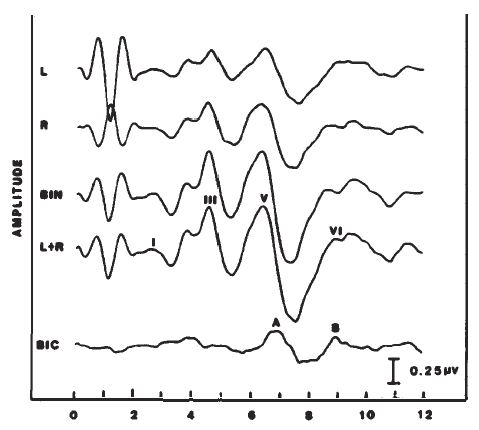
The difference between the monaural and binaural responses also forms the basis for measurement of the so-called binaural interaction potential (Figure 20). The left and right monaural responses are added (forming a predicted binaural response), and the binaural response is subtracted from this sum (Dobie & Berlin, 1979; Dobie & Norton, 1980). This difference potential is associated with Waves V-VII and is attributed to neurons that are shared by the left and right brainstem auditory pathways. The clinical utility of this component has not been established and is hampered by the low amplitude of the binaural interaction potential and its sharp dependence on waveform morphology of the monaural responses (Fowler & Swanson, 1988).
Figure 20. Binaural (BIN) versus monaural ABRs (L and R) and the derivation (i.e., BIN - [L + R]) of the binaural interaction component (BIC, demarked by Peaks A and B).
Recording Parameters
Recording techniques are selected to enhance the SNR of the auditory nerve and brainstem potentials, which typically are less than 1 V in amplitude and are buried in 10 or more V of noise. The following factors can influence the detectability and quality of the ABR: (a) electrode configuration, (b) amplification (including differential amplification), (c) filtering, (d) response averaging, and (e) artifact rejection.
Electrode Montage. Early studies of the ABR and its clinical utility relied mainly on recordings from electrodes placed on the vertex and the earlobe/mastoid of the stimulated ear with a ground on the nasion, forehead, or opposite earlobe or mastoid. The placement of electrodes on the forehead at hairline and the ipsilateral mastoid or earlobe (with the ground electrode typically placed on the contralateral mastoid) currently is popular. This montage avoids problems of affixing electrodes to skin with hair and yields similar, although not identical, results to the vertex-tomastoid montage (Beattie, Beguwala, Mills, & Boyd, 1986). An electrode on the vertex or forehead picks up the primary brainstem waves as positive potentials relative to ground, and these sites provide optimal pickup of the ABR (van Olphen, Rodenburg, & Verway, 1978). Whether the waves are traced as positive (as in Figure 14) or negative deflections (as in Figure 6) is a matter of how the electrodes are connected to the amplifier. Although no site on the head is totally inactive for the ABR (Terkildsen, Osterhammel, & Huis int Veld, 1974), a cephalic reference site is preferred as it provides for superior noise suppression because the amount and nature of the noise to both differential amplifier inputs will be similar (compared to a noncephalic reference, such as the neck). Because the earlobe/mastoid site is active for the eighth nerve potential, the AP is recorded primarily as a large negative wave but combines with the brainstem potentials via amplifier inversion to form a peak of the same apparent polarity as the brainstem components, as illustrated in Figure 21. Although different electrode placements may enhance various components of the ABR, small differences in placement will have little effect (Martin & Moore, 1977).
Figure 21. Derivation of the ipsilaterally recorded ABR (i.e., recorded between vertex and ipsilateral mastoid. Simulated from two-channel recording with the contralateral recording taken as an estimate of vertex pickup and the transverse derivation taken as an estimate of the mastoid pickup.)
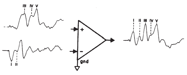
EP test systems with two or more channels permit simultaneous recording from multiple montages. For clinical purposes, a contralateral recording montage is frequently used. The vertex/forehead inputs are tied together and electrodes from each earlobe/mastoid are connected individually to each channel. As shown in Figure 22, Wave I is absent or substantially attenuated in the contralateral recording, although the negative deflection following Wave I may remain prominent at high intensities. The amplitude differences diminish for later waves and slight latency differences may be seen, with respect to the ipsilaterally recorded ABR (e.g., see data of Creel, Garber, King, & Witkop, 1980). Wave V recorded contralaterally may be as much as 0.2 ms later than the ipsilaterally recorded Wave V. One application of contralateral recordings is in cases in which the IVN complex is fused in the ipsilateral recording (Figure 22); Waves IV and V are generally separated in the contralateral recording (Stockard, Stockard, & Sharbrough, 1978).
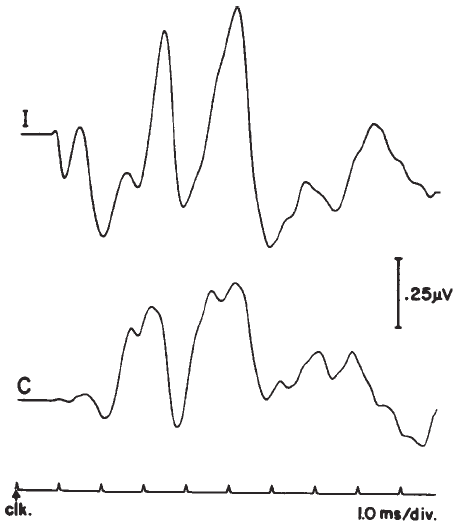
Differential effects of brainstem level pathology on the ABRs recorded contra- versus ipsilaterally have been suggested (Hashimoto, Ishiyama, & Tozuka, 1979), but some caution is needed in interpreting the responses recorded under these conditions. Such recordings do not provide independent views of the two sides of the brainstem. At most, some degree of sidedness seems probable only for Waves I–III, representing activity from the eighth nerve and, most likely, the cochlear nuclei (Durrant, Shelhamer, Fria, & Ronis, 1981). Centrally, the generators of the responses are too close together to be resolved easily in far-field recordings. Another use of two-channel recordings is to take the difference between channels (see Figure 21). This method gives the transverse derivation, which yields the same results as recording differentially between earlobes/mastoids. Although it emphasizes the pickup of auditory nerve and low brainstem potentials (Durrant, Shelhamer, Fria & Ronis, 1981), this derivation is not a substitute for ECochG because it actually does little to improve the SNR for Wave I, which is the primary problem with recording Wave I (Durrant, 1986).
Filter Bandwidth. The filter bandwidth for the ABR is selected to prevent aliasing effects on the recorded signal and to reject physical and physiological noise falling outside the spectrum of the ABR. For normal subjects, the potentials elicited by high intensity stimuli are composed of frequencies between 50 and 1000 Hz (Kevanishvili & Aponchenko, 1979), but, as the intensity of the eliciting stimuli decreases, the potentials may be composed of lower frequency components (Elberling, 1979a). Raising the cutoff of an analog high pass filter stabilizes the baseline but also decreases the latencies of the component waves and reduces their amplitudes (see analog data in Figure 23). Abnormal responses may also be composed of lower frequencies than are normal responses, so there is no one filter setting equally applicable in all situations. Current practices suggest that the high pass filter cutoff (i.e., 3 dB down point) should not exceed 100 Hz for single stage passive filters (i.e., 6 dB/octave rolloffs). The cutoff should be lowered when using filters with steeper slopes, when measuring responses from infants, and when low frequency stimuli are used. The cutoff also should be lowered and the sampling epoch extended to 20 ms when recording responses to low frequency stimuli because the low frequency content of the ABR is relatively greater than in the case of high frequency stimuli or clicks (Suzuki & Horiuchi, 1977).
Figure 23. Effects of analog (X) versus digital (O) filtering on the ABR. Analog filter settings are for a Grass recording amplifier (i.e., half-voltage cutoffs of a passive filter with initial settings of 30–3000 Hz). From Effects of Analog and Digital Filtering on Brainstem Auditory Evoked Potentials by J.R. Boston and P.J. Ainslie, 1980, Electroencephalography and Clinical Neurophysiology, 48, p. 362. Copyright 1980 by Elsevier Scientific Publishers. Reprinted by permission.
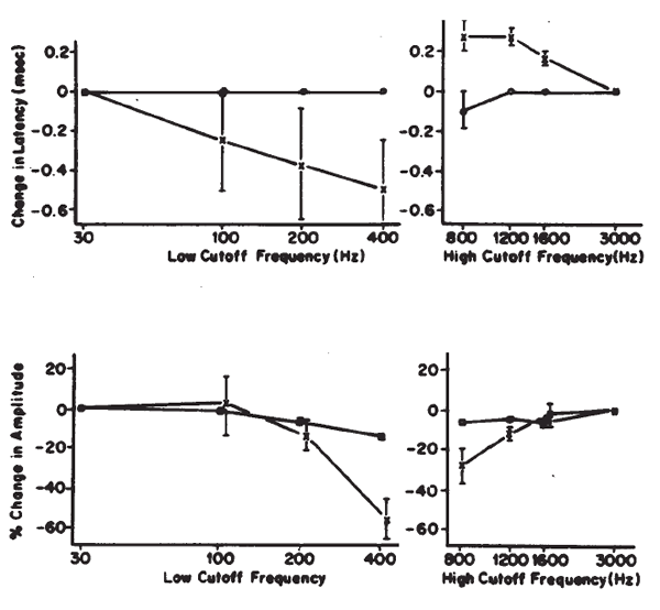
Reducing the low pass cutoff of an analog filter smoothes the responses but may increase their latencies (see analog data in Figure 23). As a consequence, cutoff frequencies below 1600 Hz are seldom used, with 3000 Hz representing a typical cutoff frequency.
Because analog filters cause phase distortion and, therefore, bias latency values, there is growing interest in the use of zero phase shift digital filtering. These filters achieve narrower bandwidths without the temporal distortion of analog filters (Boston & Ainslie, 1980; Domico & Kavanaugh, 1986). Because the filtering is much sharper, better SNRs can be obtained with less waveform distortion (although this depends on the specific filter function used). A comparison of the effects of analog versus digital filtering is shown in Figure 23.
Few commercially available systems provide the capability of digital band-pass filtering, although most provide some form of digital smoothing. Thus, analog filtering with active filter networks and 12 dB/octave rolloffs are prevalent among manufactured equipment. Despite the criticisms above, it should be recognized that adequate ABRs can be measured with appropriate analog filter settings. If more than one set of filter conditions is used routinely, however, then separate norms should be collected for each. The discussion above emphasizes the fact that response wave forms can be altered by the filter response, and thus, the use of very narrow filter bandwidths is not recommended.
Sampling Variables. The number of sweeps of the signal that must be averaged to produce a repeatable ABR is determined by various factors (e.g., stimulus intensity, subject state, and auditory sensitivity). For example, when working at relatively low stimulus levels, it may be useful to increase the number of sweeps because the amplitude of the ABR decreases with decreasing intensity. The exact number of sweeps is perhaps less important than is the reproducibility of the averaged responses for identical stimulus conditions. There should be essentially no reproducibility between responses obtained under stimulus versus nonstimulus conditions. It is advisable to repeat each condition at least once and occasionally to include nonstimulus or control conditions at intervals throughout the test session, particularly in noisy cases. In most instances, it is the examiner's pattern recognition ability that is ultimately responsible for judging the response. The repeatability of events is easier to judge than is the occurrence of isolated events. Additionally, comparisons of tracings across stimulus conditions can be helpful. For example, the peaks of the ABR are expected to shift in a fairly predictable manner as intensity changes (see Figures 16 and 17a).
Sampling rate is important because it determines the temporal resolution of the waveform and, together with the number of points sampled, the duration of the recorded epoch. Throughout the intensity range, the click-elicited ABR is generally contained within a time window of 10 ms (see Figures 14 and 16). With this window and 256 data points, there will be 40 µs temporal resolution (dwell time), which is more than sufficient, although windows up to 20 ms (80 µs resolution with 256 data points) are also adequate for ABR work. These longer time windows are necessary for evaluations of ABR thresholds, especially for low frequency stimuli, because of the long latencies of Wave V under these conditions. In general, longer windows are recommended for audiological evaluations so that the desired response can fall within the time frame of the analysis.
Subject/Nonpathologic Variables
Subject State. The ABR is relatively unaffected by changes in subject state, including natural and sedated sleep (Amadeo & Shagass, 1973; Sohmer, Gafni, & Chisin, 1978) and attention (Picton & Hillyard, 1974). As a consequence, ABRs of sedated subjects can be compared to norms established in unsedated subjects (Stockard, Stockard, & Sharbrough, 1978). For young children, and older children and adults who cannot relax, sedation should be available after clearance by the patient's physician. Immediate accessibility to emergency medical care is necessary to deal with any untoward side effects.
Anesthesia does not alter substantially the latencies or amplitudes of the potentials unless the core temperature of the body is lowered below 33 degrees Centigrade, in which case the latency of Wave V will be prolonged. Reduced temperature prolongs the absolute and relative latencies of all the waves (Stockard, Sharbrough, & Tinker, 1978). Alcohol also can increase the latency of Wave V, apparently due to an induced decrease in core temperature (Squires, Chu, & Starr, 1978).
Age and Gender. Maturational changes during early life are reflected in age-related changes in the ABR. The data presented in Figure 24, based on data from newborns (Cevette, 1984), show maturational changes in Waves III and V through the 18th month. As a consequence, ABR evaluations in premature infants and newborns require the use of age-adjusted norms and necessitate the use of a wider analysis window (e.g., 15–20 ms) than is typically used for adults (e.g., 10 ms).
Figure 24. ABR Wave V latencies and I–V interpeak latencies at indicated nHLs versus conceptual age. Conceptual ages in months (too) are actually 44 weeks (wk) + the indicated number of months. Horizontal bars above each data point demark latencies that are 2 standard deviations (sd) above the means (N = 580 newborns). From Auditory Brainstem Response Testing in the Intensive Care Unit by M.J. Cevette, 1984, Seminars in Hearing, 5, p. 62. Copyright 1984 by Thieme Medical Publishers. Adapted by permission.
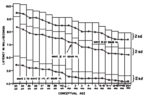
Throughout childhood the ABR changes little, but in adolescence, males begin to develop longer Wave V latencies than females, which by adulthood amounts to an average intersex difference of approximately 0.2 ms (Rowe, 1978). Additionally, females display slightly larger Wave V amplitudes than do males (Jerger & Hall, 1980). Thus, separate norms are suggested for the interpretation of the ABR in males versus females for neurologic diagnostic purposes. Because there is considerable overlap between the distributions of ABR latencies for the two sexes, however, any allowance for gender must be applied judiciously.
As adult subjects age, amplitudes of the waves may decrease and reproducibility of responses may deteriorate. The consensus of experimental evidence shows that absolute latencies of Waves I, III, and V are 0.1 to 0.2 ms longer for subjects aged 50 years and older than for those aged 20–30 years. Data regarding the influence of age on interwave latency are inconclusive but also suggest that there may be an age-related prolongation of 0.1 to 0.2 ms for the I–V interpeak interval (Chu, 1985; Rosenhall, Bjorkman, Pederson, & Kall, 1985). Age-related changes may be confounded by the presence of sensory hearing loss. Age and hearing loss appear to have opposite effects on interwave latency and similar but nonadditive effects on absolute latency. When the threshold at 4000 Hz is 50 dB HL or less, the main determinant of Wave V latency is age. When the hearing loss at 4000 Hz exceeds 50 dB HL, both age and hearing loss contribute to latency prolongations, but the major factor is hearing loss (Hyde, 1985). Thus, it is desirable to have comparative data for adults over the age of 50 years who have no more than a mild cochlear hearing loss at 4000 Hz (Brewer, 1987). For elderly adults whose threshold at 4000 Hz exceeds the mild hearing loss range, the effects of aging and hearing loss on absolute latency should be considered.
Pathologic Variables
Conductive Hearing Loss. Conductive hearing losses cause sound energy to be attenuated through the outer or middle ear. Such losses will prolong the latencies of all the waves of the ABR due to the effective lowering of the stimulus level. The evaluation of the ABR is easier and the interpretation more precise if conductive lesions are identified or resolved before the ABR is measured. Thus, otoscopic examination, immittance testing, and air and bone conduction audiometry are valuable for a thorough ABR examination if the purpose is for neurologic diagnosis.
Conductive hearing losses prolong the latencies of the waves without greatly affecting the I–V interpeak latency value and cause essentially the same degree of latency shift at all stimulus levels (Fria, 1980; Mendelson, Salamy, Lenoir, & McKean, 1979). Thus, the latency-intensity function for a subject with a conductive hearing loss is shifted along the intensity axis by essentially the amount of the conductive hearing loss (Figure 25). In addition, the waves prior to Wave V may be lost, as is generally the case with low level stimuli. There also are exceptions to the parallel shift of the latency-intensity function, for instance in cases of conductive losses that are not flat across frequency. In these cases, the latency-intensity function may be altered because the configuration of the hearing loss produces shifts in the cochlear region that dominate the response (Gorga, Reiland, & Beauchaine, 1985).
Figure 25. Example of the effects of conductive pathology on latencies of ABR Waves I, III, and V. Stippled area represents ± 2 standard deviations of latencies for normal hearing subjects.
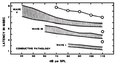
Some ostensible conductive hearing losses can arise from nonpathologic problems that can be avoided. The most common causes are ear canal collapse under earphones and slippage of the earphones during the testing. Collapsing ear canals can be dealt with most accurately and effectively with the use of insert earphones. Alternative procedures may include using an open earmold, an earphone with a circumaural cushion, or holding the earphone near (but not against) the ear. Such procedures may affect the stimulus spectrum and, accordingly, the response latencies. Although this may compromise the judgment of normalcy of the absolute latencies, reasonably accurate evaluations of interwave latencies and interaural differences can be made by testing both ears in the same manner. Earphone slippage can be detected by repeating the first test condition. If the latencies of the waves are longer on the final response, the earphone has probably slipped from its proper placement over the ear (Noffsinger & Fowler, 1983).
Cochlear Hearing Loss. The ABR may be greatly influenced by cochlear hearing loss. The overall effect is dependent on the severity and configuration of the loss, as well as the frequency composition of the stimulus. Although broad band in nature, the spectrum of the click is shaped primarily by the response characteristics of the earphone. A TDH-49 earphone, for example, has a resonance peak at about 4000–6000 Hz, which boosts the energy in that frequency range by about 10 dB. This resonance peak, the band-pass characteristics of the outer and middle ear, and the fact that the cochlea produces more synchronous responses at the basal end, lead to ABR latencies that depend on the status of high frequency neurons, at least for click stimulation.
Wave V latencies in subjects with cochlear hearing losses are essentially equivalent to those collected at the same nHL in normal hearing subjects (Selters & Brackmann, 1977) as long as these stimuli are at least 20 dB above the threshold at 4000 Hz, the configuration of the hearing loss is not steeply sloping, and the loss is no greater than mild to moderate in severity. Latency-intensity functions for these subjects also converge on those of normal hearing subjects at high intensity levels, as shown for one subject in Figure 26. (In this case the hearing loss was fairly flat in configuration and of a moderate degree.) Hearing losses confined to the low frequencies have no appreciable effect on Wave V latencies.
Figure 26. Example of the effects of cochlear pathology on latencies of ABR Waves I, III, and V as shown by circles. Stippled area represents ± 2 standard deviations of latencies for normal-hearing subjects.
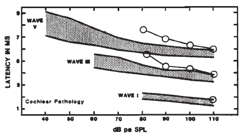
Precipitously sloping high frequency losses of moderate severity, however, cause increased latencies (Bauch & Olsen, 1986; Coats & Martin, 1977; Gorga, Reiland, & Beauchaine, 1985; Gorga, Worthington, Reiland, Beauchaine, & Goldgar, 1985). Presumably this is because of both the added time for the traveling wave to reach more normal regions of the cochlea and the reduction in stimulus intensity at the effective stimulating frequencies of the resonant peak of the earphone. Additionally, it should be recognized that the effects of high frequency hearing loss may not be identical for all components of the ABR (Coats & Martin, 1977; Fowler & Noffsinger, 1983; Keith & Greville, 1987). Clearly, for neurologic diagnostic purposes, the pure tone audiogram would be useful for accurate interpretation of the ABR evaluation.
Several methods have been proposed to account for the latency delay introduced by cochlear hearing losses when attempting to screen for retrocochlear lesions. One method is to identify Wave I through the normal electrode configuration or by placement of the reference electrode in the ear canal. Then it can be determined if the I–V interpeak latency difference is within normal limits. For cochlear hearing losses, the I–V interpeak latency difference may be normal or slightly shorter than normal (Coats & Martin, 1977). Nevertheless, the I–III interpeak latency interval can be prolonged slightly in cochlear hearing losses (with concomitant shortening of the III–V interval), even when the I–V interpeak latency difference is within normal limits (Fowler & Noffsinger, 1983).
Various corrections for Wave V latency have been suggested to take into account degree of peripheral loss (Hyde & Blair, 1981; Selters & Brackmann, 1977). Alternatively, reference data can be collected on persons with different degrees and configurations of cochlear hearing loss. Finally, tone pip stimuli or ipsilateral masking can be used to limit the response to equivalent response areas in normal and cochlear-impaired subjects (Eggermont & Don, 1980; Kileny, Schlagheck, & Spak, 1986). Because of insufficient data comparing these methods, there is no clear method of choice at this time.
Diagnostic Interpretation of the ABR Evaluation
There are two general uses of the ABR: threshold estimation and identification of auditory nerve and brainstem lesions. Otoneurologically oriented evaluations of the ABR are the focus of this section. Several variables preclude the specification of a precise procedure or method to analyze the ABR. First, the ABR must be interpreted in the context of other available information, such as history, results of audiologic evaluation, and findings of physical examination. Second, the auditory system is complex, and each wave of the ABR has multiple generators. Third, lesions vary in their size and location. Finally, different pathologies that cause lesions at the same level may have similar effects on the ABR (e.g., acoustic tumor and vascular compression of the eighth nerve). The consequence of these factors is that there is no one ABR pattern that is uniquely characteristic of a given pathology, for example, acoustic tumor versus vascular compression of the eighth nerve or multiple sclerosis versus brainstem infarct. This is true for any audiologic test that is used to indicate site of lesion. There is, however, a general relationship between level of lesion and the effects of the lesion on the ABR.
The presence of a peripheral hearing loss may confound the interpretation of wave forms in precisely those patients for whom the results of the ABR evaluation are most important. If hearing is symmetrical and nearly normal (assuming no other symptoms of neurologic consequence), suspicion of a retrocochlear pathology is low in comparison to the case in which there is a unilateral hearing loss and asymmetrical scores on other auditory tests. The latter case, however, is one in which there may be poor waveform morphology and prolonged wave latencies because of the peripheral hearing loss. There are reports of ABR abnormalities in 95% or more cases with acoustic neuromas (e.g., Selters & Brackmann, 1977). However, a false positive rate of as high as 30% can occur in cases with asymmetrical hearing losses (Clemis & Mitchell, 1977). Thus, a complete audiologic work-up in conjunction with the diagnostic ABR evaluation may provide more information than either evaluation alone. Accuracy, however, depends on the combined sensitivities and specificities of each test and their intercorrelation. For an extensive treatment of these factors and test performance, the reader is referred to a series of papers by Turner and his associates (Turner, Frazer, & Shepard, 1984; Turner & Nielsen, 1984; Turner, Shepard, & Frazer, 1984).
Although it is not our purpose to prescribe specific parameters for ABR evaluations, some generally useful approaches to the evaluation may serve as points of reference. For neurological diagnostic purposes, stimuli generally are presented at a sufficiently high intensity to elicit the potentials at or near their shortest latencies. That is, click stimuli should be presented at least 20 dB above the patient's threshold at 4000 Hz and/or at least at 95 dB peSPL (or approximately 60–65 dB nHL). More than one intensity level often is necessary to identify clearly individual waves and to assist in the interpretation of anomalies in the responses.
The fact that the population of neurons dominating the ABR changes across intensity has several clinical implications. First, for neurological applications, Wave V latency norms should be based on the absolute intensity of the stimulus and not on the subjective threshold (e.g., sensation level) or perceived loudness of the stimulus. Second, in cases of high frequency cochlear hearing losses, the response latencies may be prolonged because neurons originating from more apical regions will dominate the response. In other words, there will be a delay, attributable to the propagation characteristics of the traveling wave (Coats & Martin, 1977; Gorga, Reiland, & Beauchaine, 1985; Gorga, Worthington, Reiland, Beauchaine, & Goldgar, 1985). If, and only if, there is sufficient integrity of the basal region of the cochlea and there is sufficient stimulus intensity, then this effect can be overcome. Third, it is the intensity of the stimulus actually reaching the cochlea that is important. For example, increases in intensity can be used to compensate for any conductive loss that may be present.
The criteria for determining the normalcy of the ABR can be based on several characteristics of the response including: (a) absolute latencies, (b) interwave latency differences, (c) interaural latency differences, (d) absolute and relative amplitudes, (e) reproducibility of wave forms, (f) waveform templates with cross-correlation analysis, and (g) the judgment of presence versus absence of wave components. Of these, latencybased measures typically are used and are considered to be more reliable than amplitude-based measures. As in any procedure, it is necessary to develop confidence limits in order to account for the variance in the distribution of scores of normal subjects.
Absolute Latencies. Comparing the wave latencies to the range of normal values is the most basic method for evaluating an ABR and yet it is the most vulnerable. These latencies may be affected by various pathologic (e.g., peripheral hearing loss) and non pathologic factors (e.g., age). Still, absolute latencies are the single most used parameter of the ABR evaluation and are particularly critical for interpreting findings in cases of bilateral impairment when there is no normal ear for comparison.
Interwave Latency Differences. Presumably, interpeak intervals (see Figure 15) somewhat reflect the time necessary for a nerve impulse to travel from one generator site to another (Starr & Achor, 1975). For this reason, the terms transmission time or central conduction time are often applied to interpeak intervals. Of primary interest are the intervals between Waves I and III, I and V, and III and V. These measures have the advantage of separating a Wave V delay into its more peripheral (I–III) and more central (III–V) components. Prolongation of these intervals beyond the norms is generally suggestive of retrocochlear pathology (Figure 27a). Conductive and cochlear hearing losses do not substantially affect the transmission time from Waves I to V, although prolonged I–V intervals may be observed in cases of notched cochlear hearing loss (Keith & Greville, 1987). Thus, caution must be exercised in interpreting interpeak intervals in these cases as well as in cases of unilateral or asymmetrical cochlear losses because cochlear losses can delay Wave III without a concomitant delay in Wave V (Fowler & Noffsinger, 1983) or shorten the I–V interval. A greater problem in cases of substantial hearing loss and the major limitation in the use of the I–III and I–V intervals is that Wave I may be resolved inadequately or may be undetectable. In these cases, the application of ECochG for resolving Wave I may be beneficial (Eggermont et al, 1980).
Figure 27. ABRs recorded from patients with surgically confirmed acoustic tumors. The top waveform in each panel is from a normal ear. The lower waveform in (a) shows the prolonged I–V interval from a patient with an acoustic neuroma. The lower waveform in (b) shows an absence of waves beyond Wave II from a patient with a meningioma in the cerebello-pontine angle.
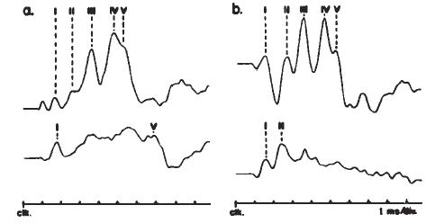
Interaural Latency Differences. Interaural latency comparisons are applied primarily to absolute Wave V latencies (Clemis & McGee, 1979; Selters & Brackmann, 1977). Normal variability of the interaural latency difference suggests that it generally should be less than 0.3–0.4 ms. (See Figure 27a for an example of an abnormal interaural latency difference.) The primary advantage of this measure is that it can be made in the absence of Wave I. Another advantage is that small retrocochlear disorders can be detected by small latency differences between ears, even when both (absolute) latencies may fall within normal limits. Each subject is his/her own control. The major disadvantage is that unilateral or asymmetrical peripheral hearing losses may create latency differences between ears, which can lead to false positive results. Here, interaural differences in the interpeak intervals may be helpful.
Amplitudes. Norms for absolute amplitudes also can be developed and used for evaluative purposes. The major limitation is that amplitudes are highly variable (Thornton, 1975). This variability is due primarily to the residual noise in the recording but also may reflect variables associated with electrode placement and variability in the potentials themselves.
An alternative to absolute amplitude measures is the use of relative amplitudes, particularly the ratio between Wave V (or IV/V) and Wave I amplitudes (Starr & Achor, 1975). This method has the potential advantage of controlling for sources of variability common to both waves. In practice the V:I ratio does not improve precision of measurement beyond that of the absolute measures, primarily due to the variability of Wave I amplitude (Durrant, 1986). Also, this measure only provides relative information about the integrity of the generators of Waves I and V and is not a measure of the overall amplitude of the ABR. The effects of stimulus parameters (e.g., see Emerson, Brooks, Parker, & Chiappa, 1982) and electrode placement must be considered. The final and most obvious problem lies in the need for both waves to be present, although Wave I can be difficult to measure in many cases presenting with hearing loss.
Reproducibility of Waveforms. The comparison of one tracing of the ABR with another gives a qualitative determination of whether or not the two traces are similar. In earlier discussions, this method was suggested as a means of judging the presence of a response. Such a comparison also can be done to assess interaural differences in wave morphology. Even in the absence of clear interaural differences in latency measures, different appearing waveforms for the two ears of stimulation could be suggestive of pathologic involvement. Although this method lacks objectivity and suffers from a lack of control over fluctuating noise levels, obvious and consistent waveform differences between ears cannot be ignored. Asymmetrical hearing loss also can cause interaural differences in the ABR waveforms.
Waveform Templates. Another approach to ABR evaluation is the use of a template for the normal response (Elberling, 1979b). The potential advantage of automated scoring procedures is to increase objectivity in ABR interpretation. This method requires the establishment of a template response from a group of normal hearing subjects and comparison of the ABR from individual patients to the template. Such a template can be formed by averaging the response from the normal group, and the comparison can be quantified by computing the correlation coefficient between the template and the individual ABR. This approach is plagued with difficulties if the SNR in the ABR under evaluation is not held constant. It requires sophisticated equipment and programming for analyses, and there may be a need to develop appropriate templates for patients of different ages, genders, and types of hearing loss. Despite the limitations, the potential advantages of these techniques are obvious and new algorithms are being evaluated (e.g. Arnold, 1985; Don, Elberling, & Waring, 1984; Elberling & Don, 1987).
Absence of Waves. The absence of waves following Wave I is a strong indication of retrocochlear pathology (Figure 27b). On the other hand, the absence of waves prior to V can result from cochlear pathology, advancing age, high physiological noise levels, or some stimulus parameters. An absence of waves following III is a strong indication of pathology affecting the rostral pons and midbrain. Waves II and IV tend to be demonstrated less reliably and are of less diagnostic significance than Waves I, III, and V. The assignment of wave numbers to the peaks of the ABR may be confounded by what appear to be extra or double peaked components. The interpretation of ABR findings can be improved by using multiple trials at different stimulus levels, different stimulus polarities, and two channel recordings.
ABRs and ABR Testing in Infants and Children
ABRs from infants differ substantially from those obtained from adults. Maturation of the auditory system is not complete at birth. Consequently, the ABR undergoes significant changes early in life. Nevertheless, ABRs have been used in screening of preterm and other high-risk neonates to identify the presence of hearing loss and to determine the need for intervention. Additionally, there has been interest in using the ABR as a basis for estimating hearing levels in patients who do not yield adequate behavioral data (e.g., due to severe mental retardation). Certain factors that must be considered in the application of ABR testing to a pediatric population are discussed below.
ABR Maturation
ABRs in infants are different from those observed in adults (Fria, 1980; Starr et al., 1977). As shown in Figure 28, waveform morphology and response latencies undergo a variety of changes as a function of age. A summary of age-related latency changes is shown in Figure 24. Wave I latencies reach adult values by 6–24 weeks, whereas latencies of Waves III and V do not attain adult values until approximately 18 months. For preterm infants, latencies of all components are prolonged compared to term infants. At about 27–30 weeks gestational age (GA) a low amplitude ABR of long latency can be recorded. Over the coming weeks, latency rapidly decreases until 35 weeks GA and then diminishes more gradually until term (38–40 weeks GA). Furthermore, during the first 18 months of life, the Wave I–V interpeak interval systematically decreases (Salamy & McKean, 1976). In preterm infants this interwave latency can be as much as 7–8 ms (i.e., at 30 weeks GA) and decreases to roughly 5.2 ms at term, in contrast to the approximate 4.0 ms of the mature response.
Figure 28. ABR from subjects of different ages, as indicated. From The Auditory Brainstem Response: Background and Clinical Applications by T.J. Fria, 1980, in Postnatal development of human brainstem life by A. Salamy and C.M. McKean, 1976, Electroencephalography and Clinical Neurophysiology, 40, p. 421. Copyright 1976 by Elsevier Scientific Publishers. Adapted by permission.
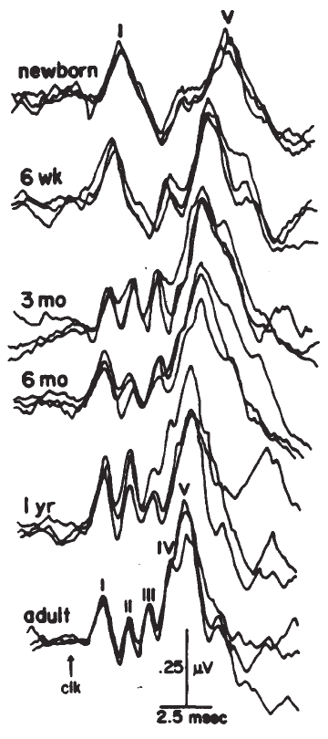
The ABR also exhibits maturational changes in terms of amplitudes of individual components (Salamy, Fenn, & Bronshvag, 1979). Waves I and III increase in amplitude until approximately 6 months of chronologic age (CA), then decrease slightly until adulthood. Wave V amplitude increases to a peak value at between 24 and 60 months CA, and then decreases slightly until adulthood.
Typically, the click-evoked ABR Wave V threshold shows little or no age-dependent effects, at least for children as young as 33 weeks conceptional age (Gorga, Reiland, Beauchaine, Worthington, & Jesteadt, 1987). When frequency-specific stimuli have been used, maturational effects vary with frequency. In general, it has been shown that when ABRs are restricted to the basal region of the cochlea, they exhibit the greatest age-related differences in threshold and latencies (Klein, 1984; Teas, Klein, & Kramer, 1982). When the responses are restricted to apical portions of the cochlea, through the use of masking or frequency-specific stimuli, the ABRs from infants are similar to ABRs from adults in terms of both VDLs and Wave V latencies (Folsom & Wynne, 1986; Klein, 1984). Consequently, interpretation of ABR studies in infants must be made in light of the stimuli used to elicit responses. The timetable for development of mature Wave V latencies, when using mid- or low-frequency stimuli, is significantly shorter than when using click stimuli (Teas et al., 1982).
Clinical Application
Failure to account for age-related differences in infant responses can result in substantial errors in hearing level estimation (up to 30 dB), particularly if stimuli are high-frequency tone pips (Klein, 1984). For example, if adult norms (for either latency or detection threshold) are used, an infant might appear to deviate substantially from the norm when, in fact, the infant's responses are within the normal range for his/her age. If only click stimuli are used, response detection thresholds are relatively stable across age.
The relationship between ABR and behavioral thresholds permits accurate predictions of hearing loss. This feature is useful because it allows assessment of difficult-to-test patients who may be unable to provide voluntary responses to sound. As a consequence, hearing loss can be identified expediently permitting timely (re)habilitative intervention. It should be recognized that there are certain cases when the ABR may not accurately reflect auditory sensitivity, although these cases are extremely rare (Murray, Javel & Watson, 1985; Worthington & Peters, 1980). The interpretive accuracy of the ABR evaluation can be enhanced when it is combined with other data, such as acoustic immittance measures, behavioral audiological measures, and case history information.
Although it is beyond the scope of this writing to delve into the details of strategies and protocols for ABR evaluations directed toward auditory assessment, a brief overview of the typical procedure can be given. An intensity series usually is conducted. Wave V is tracked down to the VDL, which is generally within 10 dB of the behavioral threshold, at least for the higher frequencies (Gorga, Reiland, & Beauchaine, 1985; Jerger & Mauldin, 1978). The latency-intensity function also can be useful in such assessments (Coats & Martin, 1977, Gorga, Reiland, & Beauchaine, 1985; Gorga, Worthington, Reiland, Beauchaine, & Goldgar, 1985), but the VDL is relied on most heavily for threshold estimation. This procedure usually is repeated for each ear, using stimuli of different frequencies, although such evaluations may be initiated with the click.
Sedation
Infants and young children up to 7 years of age (or older, if uncooperative) typically require some form of sedation in order to improve the SNR and to permit sufficient time to complete the test. Natural sleep is typically sufficient for infants up to 6 months of age, although it is usually safe to sedate younger children (Fria, 1980).
The most common sedative used is chloral hydrate, although others (e.g., secobarbital and a “cocktail” of Demerol, phenergan, and thorazine) are often used. Medical supervision of the administration of the sedative and availability of medical personnel for emergency intervention is required. The evaluation must be carefully coordinated with the child's parents or guardians so that the child will be appropriately sedated at the time of the test. For example, it might be useful to deny a child his/her nap during the day of the test. ABR testing must be carried out efficiently because sedation wears off quickly. It is also important to remember that these sedatives differ from anesthesia, so that unnecessary stimulation (e.g., excessive or abrupt body movement) should be avoided. Finally, in some cases where no sedation of any form is successful, general anesthesia may be the only recourse. In electing to test under general anesthesia, the risk-benefit equation should be evaluated carefully. Guidelines for the use of sedation and general anesthesia in pediatric patients have been formulated by the American Academy of Pediatrics (1985).
Other Auditory Evoked Potentials
The focus of this tutorial has been on the ECochGm and ABR, which are the earliest segments of the electric response of the brain to sound. The entire AEP may last several hundred milliseconds or longer (Figure 29). Estimates of hearing sensitivity, using electrophysiologic measures, have not been limited to the short latency responses. For example, responses in the 10–50 ms epoch, known as the middle latency responses (MLRs), are recorded easily with minor parametric and procedural changes from the ABR recording and are reportedly useful for obtaining near threshold information for low frequency stimuli (Mendel & Wolf, 1983). The 40-Hz event-related or steady-state potential has been reported to be useful for estimating low frequency sensitivity as well (Galambos, Makeig, & Talmachoff, 1981) although response variability as a function of sleep state is problematic. Late or long latency cortical EPs have a long history of clinical application (see Reneau & Hnatiow, 1975). Although the late responses can provide reasonably good estimates of hearing thresholds, they are vulnerable to subject state variables, such as level of arousal or even state of attention (Schwent, Hillyard, & Galambos, 1976) and are not currently used to estimate threshold. The cortical potentials have been of interest because of their presumed relationship to the perceptual attributes of sound and interhemispheric differences and because of their various neurologic and psychiatric applications.
Figure 29. Auditory evoked potential analyzed on logarithmic time-base to reveal the component potentials with approximately equal weighting and categorized in arbitrary but commonly used time windows of short- (SLR), middle- (MLR), and long- (LLR) latency responses. (Figure modified and redrawn from Michelini et al., 1982.)
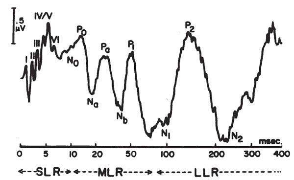
The MLRs and later responses are beyond the scope of this writing, but it is important to recognize that there may be useful information from activity recorded beyond the time window discussed in this tutorial. Additionally, there are other phenomena and applications related to the short latency potentials that were not covered in this document. These topics and their kernel references include: the frequency following response and the SN-10 response (Davis, 1976), hearing aid selection based on ABR measures (Beauchaine, Gorga, Reiland & Larson, 1986; Gorga, Beauchaine, & Reiland, 1987; Hecox, 1983), ABR monitoring during surgery (Grundy, Janetta, Procopio, Lina, Boston, & Doyle, 1981; Moller & Janetta, 1983), and the use of ABR evaluation to assist in outcome prediction for the comatose patient and as a part of the assessment of brain death (Brewer & Resnick, 1984; Hall, Mackey-Hargadine, & Kim, 1985; Hall & Tucker, 1986; Seales, Rossiter, & Weinstein, 1979).
The intent of this tutorial was to provide an overview for clinicians of the short latency AEPs. The influence of instrumental, stimulus, and subject variables were reviewed in the context of their effects on the clinical application of AEPs. Both the strengths and limitations of ECochG and ABR measures for threshold determination and otoneurologic diagnosis were discussed. The applications of these techniques are within the scope of practice of clinical audiologists, both from traditional and contemporary perspectives. This tutorial is intended to serve as a helpful tool for those clinical audiologists using these techniques and to prepare them for future developments in this field.
References
Achor, L. J., & Starr, A. (1980a). Auditory brainstem responses in the cat I: Intracranial and extracranial recordings. Electroencephalography and Clinical Neurophysiology, 48, 154–173.
Achor, L. J., & Starr, A. (1980b). Auditory brainstem responses in the cat II: Effects of lesions. Electroencephalography and Clinical Neurophysiology, 48, 174–190.
Amadeo, M., & Shagass, C. (1973). Brief latency clickevoked potentials during waking and sleep in man. Psychophysiology, 10, 244–250.
American Academy of Pediatrics. (1985). Guidelines for the elective use of conscious sedation, deep sedation, and general anesthesia in pediatric patients. Pediatrics, 76, 317–321.
Aran, J. M. (1978). Contributions of electrocochleography to diagnosis in infancy. An 8 year survey. In S. E. Gerber & G. T. Mencher (Eds.), Early diagnosis of hearing loss (pp. 215–242). New York: Grune & Stratton.
Arnold, S. A. (1985). Objective versus visual detection of the auditory brainstem response. Ear and Hearing, 6, 144–150.
Bauch, C. D., & Olsen, W. O. (1986). The effect of 2000–4000 Hz hearing sensitivity on ABR results. Ear and Hearing, 7, 314–317.
Beagley, H. A. (1974). Can we use the cochlear microphonic in electrocochleography? Revue de Laryngologie, 95, 531–536.
Beattle, R. C., Beguwala, F. E., Mills, D. M., & Boyd, R. L. (1986). Latency and amplitude effects of electrode placement on the early auditory evoked response. Journal of Speech and Hearing Disorders, 51, 63–70.
Beauchaine, K. A., Gorga, M. P., Reiland, J. K., & Larson, L. L. (1986). The application of auditory brainstem response measurements to the selection of hearing aids: Preliminary data. Journal of Speech and Hearing Research, 29, 120–128.
von Bekesy, G. (1974). Experiments in hearing. New York: McGraw-Hill.
Berlin, C. I., Cullen, J. K., Ellis, M. S., Lousteau, R. J., Yarbrough, W. M., & Lyons, G. D. (1974). Clinical application of recording human VIIIth nerve action potentials from the tympanic membrane. Transactions of the American Academy of Ophthalmology and Otolaryngology, 78, 401–410.
Berlin, C. I., & Gorga, M. I. (1976). Extratympanic clinical electrocochleography with clicks. In R. J. Ruben, C. Elberling, & G. Salomon (Eds.), Electrocochleography (pp. 457–469). Baltimore: University Park Press.
Berlin, C. I., Gondra, M. I., & Casey, D. (1978). Bone conduction electrocochleography: Clinical applications. Laryngoscope, 88, 56–763.
Binnie, C. D., Rowan, A. J., & Gutter, T. (1982). A manual of electroencephalographic technology. Cambridge, England: Cambridge University Press.
Boston, J. R., & Ainslie, P. J. (1980). Effects of analog and digital filtering on brainstem auditory evoked potentials. Electroencephalography and Clinical Neurophysiology, 48, 361–364.
Brewer, C. C. (1987). Electrophysiologic measures. In H. G. Mueller & V. C. Geoffrey (Eds.), Communication disorders in aging (pp. 334–380). Washington, DC: Gallaudet University Press.
Brewer, C. C., & Resnick, D. M. (1984). The value of BAEP in assessment of the comatose patient. In R. H. Nodar & C. Barber (Eds.), Evoked potentials II (pp. 578–581). Boston: Butterworth Publishers.
Buchwald, J. S., & Huang, C. M. (1975). Far-field acoustic response: Origins in the cat. Science, 189, 382–384.
Campbell, K. C. M., & Abbas, P. J. (1987). The effect of stimulus repetition on the auditory brainstem response in tumor and nontumor patients. Journal of Speech and Hearing Research, 30, 494–502.
Cann, J., & Knott, J. (1979). Polarity of acoustic click stimuli for eliciting brainstem auditory evoked responses: A proposed standard. American Journal of Electroencephalography and Technology, 19, 125–132.
Cevette, M. J. (1984). Auditory brainstem response testing in the intensive care unit. Seminars in Hearing, 5, 57–68.
Chu, N. S. (1985). Age related changes in the brainstem auditory evoked potentials. Electroencephalography and Clinical Neurophysiology, 62, 431–436.
Clemis, J. D., Ballad, J., & Killion, M. C. (1986). Clinical use of an insert earphone. Annals of Otology, Rhinology, and Laryngology, 95, 520–524.
Clemis, J. D., & McGee, T. (1979). Brainstem electric response audiometry in the differential diagnosis of acoustic tumors. Laryngoscope, 89, 31–42.
Clemis, J. D., & Mitchell, C. (1977). Electrocochleography and brainstem responses used in the diagnosis of acoustic tumors. Journal of Otolaryngology, 6, 447–459.
Coats, A. C. (1974). On electrocochleographic electrode design. Journal of the Acoustical Society of America, 56, 708–711.
Coats, A. C. (1981). The summating potential and Meniere's disease. Archives of Otolaryngology, 107, 199–208.
Coats, A. C. (1983). Instrumentation. In E. J. Moore (Ed.), Bases of auditory brainstem evoked responses (pp. 197–220). New York: Grune & Stratton.
Coats, A. C. (1986). Electrocochleography: Recording techniques and clinical applications. Seminars in Hearing (Electrocochleography), 7, 247–266.
Coats, A. C., & Martin, J. L. (1977). Human auditory nerve action potentials and brainstem evoked responses. Archives of Otolaryngology, 103, 605–622.
Creel, D., Garber, S. R., King, R. A., & Witkop, C. J. (1980). Auditory brainstem anomalies in human albinos. Science, 209, 1253–1255.
Cullen, J. K., Ellis, M. S., Berlin, C. I., & Lousteau, R. J. (1972). Human acoustic nerve action potential recordings from the tympanic membrane without anesthesia. Acta Otolaryngologica, 74, 15–22.
Dallos, P. (1973). The auditory periphery. New York: Academic.
Davis, H. (1976). Principles of electric response audiometry. Annals of Otology, Rhinology, and Otolaryngology, 85(Suppl. 28), 1–96.
Dobie, R. A., & Berlin, C. I. (1979). Binaural interaction in brainstem-evoked responses. Archives of Otolaryngology, 105, 391–398.
Dobie, R. A., & Norton, S. J. (1980). Binaural interaction in human auditory evoked potentials. Electroencephalography and Clinical Neurophysiology, 49, 303–313.
Domico, W. D., & Kavanaugh, K. T. (1986). Analog and zero phase-shift digital filtering of the auditory brainstem response waveform. Ear and Hearing, 7, 377–382.
Don, M., & Eggermont, J. J. (1978). Analysis of the clickevoked brainstem potentials in man using high-pass noise masking. Journal of the Acoustical Society of America, 63, 1084–1092.
Don, M., Eggermont, J. J., & Brackmann, D. E. (1979). Reconstruction of the audiogram using brainstem responses and high-pass noise masking. Annals of Otology, Rhinology, and Laryngology, 88(Suppl. 57), 1–20.
Don, M., Elberling, C., & Waring, M. (1984). Objective detection of averaged auditory brainstem responses. Scandinavian Audiology, 13, 219–228.
Durrant, J. D. (1977). Study of a combined noninvasive ECochG and BSER recording technique. Journal of the Acoustical Society of America, 62, S87.
Durrant, J. D. (1983). Fundamentals of sound generation. In E. J. Moore (Ed.), Bases of auditory brainstem evoked responses (pp. 15–49). New York: Grune Stratton.
Durrant, J. D. (1986). Combined ECochG-ABR versus conventional ABR recordings. Seminars in Hearing (Electrocochleography), 7, 289–305.
Durrant, J. D., Gabriel, S., & Walter, M. (1981). Psychophysical tuning functions for brief stimuli: Preliminary report. American Journal of Otolaryngology, 2, 108–113.
Durrant, J. D., & Lovrinic, J. H. (1984). Bases of hearing science (2nd ed.). Baltimore: Williams & Wilkins.
Durrant, J. D., Shelhamer, M., Fria, T. J., & Ronis, M. L. (1981). Examination of the sidedness of the brainstem auditory evoked potential. Paper presented at the biennial symposium of the international response audiometry study group, Bergamo. Italy.
Eggermont, J. J. (1976a). Analysis of compound action potential responses to tone bursts in the human and guinea pig cochlea. Journal of the Acoustical Society of America, 60, 1132–1139.
Eggermont, J. J. (1976b). Electrocochleography. In W. D. Keidel & W. D. Neff (Eds.), Handbook of sensory physiology, Vol. V/3: Auditory system-Clinical and special topics (pp. 625–705). Berlin: Springer-Verlag.
Eggermont, J. J., & Don, M. (1980). Analysis of the clickevoked brainstem potentials in humans using high-pass noise masking. II. Effect of click intensity. Journal of the Acoustical Society of America, 68, 1671–1675.
Eggermont, J. J., Don, M., & Brackmann, D. E. (1980). Electrocochleography and auditory brainstem electric responses in patients with pontine angle tumors. Annals of Otology, Rhinology, and Laryngology, 89(Suppl. 75), 1–19.
Eggermont, J. J., Odenthal, D. W., Schmidt, P. H., & Spoor, A. (1974). Electrocochleography: Basic principles and clinical application. Acta Otolaryngologica(Suppl. 316), 1–84.
Elberling, C. (1979a). Auditory electrophysiology: Spectral analysis of cochlear and brainstem evoked potentials. Scandinavian Audiology, 8, 57–64.
Elberling, C. (1979b). Auditory electrophysiology: The use of templates and cross correlation functions in the analysis of brainstem potentials. Scandinavian Audiology, 8, 187–190.
Elberling, C., & Don, M. (1987). Threshold characteristics of the human auditory brainstem response. Journal of the Acoustical Society of America, 81, 115–121.
Elberling, C., & Salomon, G. (1973). Cochlear microphonics recorded from the ear canal in man. Acta Otolaryngologica, 75, 489–495.
Emerson, R. G., Brooks, E. B., Parker, S. W., & Chiappa, K. H. (1982). Effects of click polarity on brainstem auditory evoked potentials in normal subjects and patients: Unexpected sensitivity of Wave V. Annals of the New York Academy of Science, 288, 710–721.
Ferraro, J. A. (Ed.). (1986). Seminars in Hearing (Electrocochleography) , 7, 241-337.
Ferraro, J. A., Arenberg, I. K., & Hassanein, R. S. (1985). Electrocochleography and symptoms of inner ear dysfunction. Archives of Otolaryngology, 111, 71–74.
Ferraro, J. A., & Ferguson, R. (in press). Tympanic ECochG and conventional ABR: A combined approach for the identification of Wave I and the I–V interwave interval. American Journal of Otology.
Ferraro, J. A., Murphy, G. B., & Ruth, R. A. (1986). A comparative study of primary electrodes used in extratympanic electrocochleography. Seminars in Hearing, 7, 279–287.
Finitzo-Hieber, T., Hecox, K., & Cone, B. (1979). Brainstem auditory evoked potentials in patients with congenital atresia. Laryngoscope, 89, 1151–1158.
Folsom, R. C. (1984). Frequency specificity of human auditory brainstem responses as revealed by pure-tone masking profiles. Journal of the Acoustical Society of America, 66, 919–914.
Folsom, R. C., & Wynne, M. K. (1986). Auditory brainstem responses from human adults and infants: Restriction of frequency contribution by notched-noise masking. Journal of the Acoustical Society of America, 80, 1057–1064.
Fowler, C. G., & Noffsinger, D. (1983). The effects of stimulus repetition rate and frequency on the auditory brainstem response in normal, cochlear-impaired, and VIII nerve/brainstem-impaired subjects. Journal of Speech and Hearing Research, 26, 560–567.
Fowler, C. G., & Swanson, M. R. (1988). Binaural and monaural phasic differences in the auditory brainstem response Manuscript submitted for publication.
Fria, T. J. (1980). The auditory brainstem response: Background and clinical applications. Monographs in Contemporary Audiology, 2, 1–44.
Fria, T. J., & Doyle, W. J. (1984). Maturation of the auditory brainstem response (ABR): Additional perspectives. Ear and Hearing, 5, 361–365.
Galambos, R., Makeig, S., & Talmachoff, P. J. (1981). A 40-Hz auditory potential recorded from the human scalp. In Proceedings of the National Academy of Science (Vol. 78, pp. 2643–2647).
Geddes, L. A. (1972). Electrodes and the measurement of bioelectric events. New York: Wiley-Interscience.
Gibson, W. P. R., Moffat, D. A., & Ramsden, R. T. (1977). Clinical electrocochleography in the diagnosis and management of Meniere's disorder. Audiology, 16, 389–401.
Glattke, T. J. (1983). Short latency auditory evoked potentials. Baltimore: University Park Press.
Gorga, M. P., Abbas, P. J., & Worthington, D. W. (1985). Stimulus calibration in ABR measurements. In J. T. Jacobson (Ed.), The auditory brainstem response (pp. 49–62). San Diego, CA: College-Hill.
Gorga, M. P., Beauchaine, K. A., & Reiland, J. K. (1987). Comparison of onset and steady-state responses of hearing aids. Implications for use of the auditory brainstem response in the selection of hearing aids. Journal of Speech and Hearing Research, 30, 130–136.
Gorga, M. P., Beauchaine, K. A., Reiland, J. K., Worthington, D. W., & Javel, E. (1984). The effects of stimulus duration on ABR and behavioral thresholds. Journal of the Acoustical Society of America, 76, 616–619.
Gorga, M. P., Reiland, J. K., & Beauchaine, K. A. (1985). Auditory brainstem responses in a case of high-frequency conductive hearing loss. Journal of Speech and Hearing Disorders, 50, 346–350.
Gorga, M. P., Reiland, J. K., Beauchaine, K. A., Worthington, D. W., & Jesteadt, W. (1987). Auditory brainstem responses from graduates of an intensive care nursery: Normal patterns of response. Journal of Hearing Research, 30, 311–318.
Gorga, M. P., Worthington, D. W., Reiland, J. K., Beauchaine, K. A., & Goldgar, D. E. (1985). Some comparisons between auditory brainstem response thresholds, latencies, and the pure-tone audiogram. Ear and Hearing, 6, 105–112.
Grundy, B. L., Janetta, P. J., Procopio, P., Lina, A., Boston, J. R., & Doyle, E. (1981). Intraoperative monitoring of brainstem auditory evoked potentials. Journal of Neurosurgery, 57, 674–681.
Hall, J. W., Mackey-Hargadine, J. R., & Kim, E. E. (1985). Auditory brainstem response in the determination of brain death. Archives of Otolaryngology, 111, 613–620.
Hall, J. W., & Tucker, D. A. (1986). Sensory evoked responses in the intensive care unit. Ear and Hearing, 7, 220–232.
Harris, D. M., & Dallos, P. J. (1979). Forward masking of auditory nerve fiber responses. Journal of Neurophysiology, 42, 1083–1107.
Harris, F. J. (1978). On the use of windows for harmonious analysis with the discrete Fourier Transform. In Proceedings of the IEEE (Vol. 66, pp. 51–83).
Hashimoto, I., Ishiyama, Y., & Tozuka, G. (1979). Bilaterally recorded brainstem auditory evoked responses. Their asymmetric abnormalities and lesions of the brainstem. Archives of Neurology, 36, 161–167.
Hecox, K. E. (1983). Role of auditory brainstem responses in the selection of hearing aids. Ear and Hearing, 4, 51–55.
Hecox, K., Squires, N., & Galambos, R. (1976). Brainstem auditory evoked responses in man. I. Effect of stimulus rise-fall time and duration. Journal of the Acoustical Society of America, 60, 1187–1192.
Hoke, M., & Lutkenhoner, B. (1981). Electrophysiological findings in patients with sudden deafness: A survey. In Advances in otorhinolaryngology (pp. 83–99). Basel: S. Karger.
Hood, L. J., & Berlin, C. I. (1986). Auditory evoked potentials. Austin, TX: Pro-Ed.
Hyde, M. L. (1985). The effect of cochlear lesions on the ABR. In J. T. Jacobson (Ed.), The auditory brainstem response (pp. 133–146). San Diego, CA: College Hill Press.
Hyde, M. L., & Blair, R. L. (1981). The auditory brainstem response in neuro-otology: Perspectives and problems. Journal of Otolaryngology, 10, 117–125.
Jacobson, J. D. (Ed.). (1985). The auditory brainstem response. San Diego, CA: College-Hill Press.
Jerger, J., & Hall, J. (1980). Effects of age and sex on auditory brainstem response. Archives of Otolaryngology, 106, 387–391.
Jerger, J., & Mauldin, L. (1978). Prediction of sensorineural hearing level from the brainstem evoked response. Archives of Otolaryngology, 104, 454–461.
Jewett, D. L. (1970). Volume-conducted potentials in response to auditory stimuli as detected by averaging in the cat. Electroencephalography and Clinical Neurophysiology, 28, 609–618.
Jewett, D. L., Romano, M. N., & Williston, J. S. (1970). Human auditory evoked potentials: Possible brainstem components detected on the scalp. Science, 167, 1517–1518.
Jewett, D. L., & Williston, J. S. (1971). Auditory evoked far fields averaged from the scalp of humans. Brain, 94, 681–696.
Joint Commission on Accreditation of Hospitals. (1987). Standard PI.9: Patient care equipment. Accreditation Manual for Hospitals, 199–200.
Keith, W. J., & Greville, K. A. (1987). Effects of audiometric configuration on the auditory brainstem response. Ear and Hearing, 8, 49–55.
Kevanishvili, Z., & Aphonchenko, V. (1979). Frequency composition of brainstem auditory evoked potentials. Scandinavian Audiology, 8, 51–55.
Kileny, P., Schlagheck, G., & Spak, C. (1986). Site of lesion ABR testing with tonal stimuli. Paper presented at the annual convention of the American Speech-Language-Hearing Association, Detroit.
Klein, A. J. (1984). Frequency and age-dependent auditory evoked thresholds in infants. Hearing Research, 16, 291–297.
Kodera, K., Marsh, R. R., Suzuki, M., & Suzuki, J. (1983). Portions of tone pips contributing to frequency-selective auditory brainstem responses. Audiology, 22, 209–218.
Martin, M., & Moore, E. (1977). Scalp distribution of early (0–10 msec) auditory evoked responses. Archives of Otolaryngology, 103, 326–328.
Mauldin, L., & Jerger, J. (1979). Auditory brainstem evoked responses to bone-conducted signals. Archives of Otolaryngology, 105, 656–661.
McClelland, R. J., & McCrea, R. S. (1979). Intersubject viability of the auditory-evoked brainstem potentials. Audiology, 18, 462–471.
Mendel, M. I., & Wolf, K. E. (1983). Clinical applications of the middle latency responses. Audiology: A Journal for Continuing Education, 8, 141–155.
Mendelson, T., Salamy, A., Lenoir, M., & McKean, C. (1979). Brainstem evoked potential findings in children with otitis media. Electroencephalography and Clinical Neurophysiology, 105, 17–20.
Michelini, S., Arslan, E., Prosser, S., & Pedrielli, F. (1982). Logarithmic display of auditory evoked potentials. Journal of Biomedical Engineering, 4, 62–64.
Moller, A. R. (1986). Effect of click spectrum and polarity on round window N1N2 response in the rat. Audiology, 25, 29–43.
Moller, A. R., & Jannetta, P. J. (1982). Comparison between intracranially recorded potentials from the human auditory nerve and scalp recorded auditory brainstem responses (ABR). Scandinavian Audiology, 11, 3340.
Moller, A. R., & Jannetta, P. J. (1983). Monitoring auditory functions during cranial nerve microvascular decompression operations by direct monitoring from the eighth nerve. Journal of Neurosurgery, 59, 493–499.
Moller, A. R., Jannetta, P. J., Bennett, M., & Moller, M. B. (1981). Intracranially recorded responses from the human auditory nerve: New insights into the origin of brainstem evoked potentials (BSEP). Electroencephalography and Clinical Neurophysiology, 52, 18–27.
Moller, K., & Blegvad, B. (1976). Brainstem responses in patients with sensorineural hearing loss. Scandinavian Audiology, 5, 115–127.
Moore, E. J. (1983). Bases of auditory brainstem evoked responses. New York: Grune Stratton.
Murray, A. D., Javel, E., & Watson, C. S. (1985). Prognostic validity of auditory brainstem evoked response screening in newborn infants. American Journal of Otolaryngology, 6, 120–131.
Naunton, R. F., & Zerlin, S. S. (1976). Basis and some diagnostic implications of electrocochleography. Laryngoscope, 86, 475–482.
Noffsinger, D., & Fowler, C. G. (1983). Brainstem auditory evoked potentials: Applications in clinical audiology. Bulletin of the Los Angeles Neurological Societies, 47, 43–54.
Nuttall, A. H. (1981). Some windows with very good sidelobe behavior. IEEE Transactions on Acoustics, Speech and Signal Processing, 29, 84–91.
Nyquist, H. (1924). Certain factors affecting telegraph speed. Bell System Technical Journal, 3(2), 324–346.
Pfeiffer, R. R. (1974). Consideration of the acoustic stimulus. In W. D. Keidel & W. D. Neff (Eds.), Handbook of sensory physiology, Vol. V/l: Auditory system-Anatomy and physiology (ear) (pp. 9–38). Berlin: Springer-Verlag.
Picton, T. W., & Hillyard, S. A. (1974). Human auditory evoked potentials. II. Effects of attention. Electroencephalography and Clinical Neurophysiology, 36, 191–200.
Picton, T. W., & Hink, R. F. (1974). Evoked potentials: How? What? Why? American Journal of EEG Technology, 14, 9–44.
Picton, T. W., Ouellette, J., Hamel, G., & Smith, A. D. (1979). Brainstem evoked potentials to tonepips in notched noise. Journal of Otolaryngology, 8, 289–314.
Picton, T. W., Stapells, D. R., & Campbell, K. B. (1981). Auditory evoked potentials from the human cochlea and brainstem. Journal of Otolaryngology, 10(Suppl. 9), 1–41.
Probst, R. (1983). Electrocochleography: Using extratympanic or transtympanic methods? ORL-Journal of Otorhinolaryngology and Related Specialties, 45, 322–329.
Reneau, J. P., & Hnatiow, G. Z. (1975). Evoked response audiometry. Baltimore: University Park Press.
Rosenhall, U., Bjorkman, G., Pederson, K., & Kall, H. (1985). Brainstem auditory evoked potentials in different age groups. Electroencephalography and Clinical Neurophysiology, 62, 426–430.
Rowe, M. J. (1978). Normal variability of the brainstem auditory evoked response in young and old adult subjects. Electroencephalography and Clinical Neurophysiology, 44, 459–470.
Ruth, R. A., Lambert, R. R., & Ferraro, J. A. (in press). Electrocochleography: Methods and clinical applications. American Journal of Otology.
Ruth, R. A., Mills, J. A., & Ferraro, J. A. (in press). The use of disposable ear canal electrodes in auditory brainstem response testing. American Journal of Otology.
Salamy, A., Fenn, E., & Bronshvag, M. (1979). Ontogenesis of human auditory brainstem evoked potential amplitude. Developmental Psychology, 12, 519–526.
Salamy, A., & McKean, C. M. (1976). Postnatal development of human brainstem potentials during the first year of life. Electroencephalography and Clinical Neurophysiology, 40, 418–426.
Salt, A. N., & Thornton, A. R. (1983). The effects of stimulus rise-time and polarity on the auditory brainstem responses. Scandinavian Audiology, 13, 119–127.
Schwartz, D. M., Larson, V. D., & DeChicchis, A. R. (1985). Spectral characteristics of air and bone conduction transducers used to record the auditory brainstem response. Ear and Hearing, 6, 274–277.
Schwent, V. L., Hillyard, S. A., & Galambos, R. (1976). Selective attention and the auditory vertex potential. I. Effects of stimulus delivery rate. Electroencephalography and Clinical Neurophysiology, 40, 604–614.
Seales, D. M., Rossiter, V. S., & Weinstein, M. D. (1979). Brainstem auditory evoked responses in patients comatose as a result of blunt head trauma. Journal of Trauma, 19, 347–353.
Selters, W. A., & Brackmann, D. E. (1977). Acoustic tumor detection with brainstem electric response audiometry. Archives of Otolaryngology, 103, 181–187.
Sohmer, H., & Feinmesser, M. (1967). Cochlear action potentials recorded from the external ear in man. Annals of Otology, Rhinology, and Laryngology, 76, 427–435.
Sohmer, H., & Feinmesser, M. (1973). Routine use of electrocochleography (cochlear audiometry) on human subjects. Audiology, 12, 167–173.
Sohmer, H., & Feinmesser, M. (1974). Electrocochleography in clinical-audio logical diagnosis. Archives of Otolaryngology, 206, 91–102.
Sohmer, H., Feinmesser, M., & Bauberger-Tell, L. (1972). Routine use of cochlear audiometry in infants with uncertain diagnosis. Annals of Otology, Rhinology, and Laryngology, 81, 72–75.
Sohmer, H., Feinmesser, M., & Szabo, G. (1974). Electrocochleographic (auditory nerve and brainstem auditory nuclei) responses to sound stimuli in patients with brain damage. Electroencephalography and Clinical Neurophysiology, 37, 663–669.
Sohmer, H., Gafni, M., & Chisin, R. (1978). Auditory nerve and brainstem responses: Comparison in awake and unconscious subjects. Archives of Neurology, 35, 228–230.
Sohmer, H., & Pratt, H. (1976). Recording of the cochlear microphonic potential with surface electrodes. Electroencephalography and Clinical Neurophysiology, 40, 253–260.
Squires, K. C., Chu, N., & Starr, A. (1978). Acute effects of alcohol on auditory brainstem potentials. Science, 201, 174–176.
Staller, S. (1986). Electrocochleography in the diagnosis and management of Meniere's disease. Seminars in Hearing (Electrocochleography), 7, 267–277.
Stapells, D. R., & Picton, T. W. (1981). Technical aspects of brainstem evoked potential audiometry using tones. Ear and Hearing, 2, 20–29.
Stapells, D. R., Picton, T. W., Perez-Abalo, M., Read, D., & Smith, A. (1985). Frequency specificity in evoked potential audiometry. In J. T. Jacobson (Ed.), The auditory brainstem response (pp. 147–177). San Diego, CA: College-Hill.
Stapells, D. R., Picton, T. W., & Smith, A. D. (1982). Normal hearing thresholds for clicks. Journal of the Acoustical Society of America, 72, 74–79.
Starr, A., & Achor, L. J. (1975). Auditory brainstem responses in neurological disease. Archives of Neurology, 32, 761–768.
Starr, A., Amlie, R. N., Martin, W. H., & Sanders, S. (1977). Development of auditory function in newborn infants revealed by auditory brainstem potentials. Pediatrics, 60, 831–839.
Stockard, J. J., Sharbrough, F. W., & Tinker, J. A. (1978). Effects of hypothermia on the human brainstem auditory response. Annals of Neurology, 3, 368–370.
Stockard, J. J., Stockard, J. E., & Sharbrough, F. W. (1978). Nonpathologic factors influencing brainstem auditory evoked potentials. American Journal of Electroencephalogram Technology, 18, 177–209.
Stypulkowski, P. H., & Staller, S. J. (1987). Clinical evaluation of a new ECochG recording electrode. Ear and Hearing, 8, 304–310.
Suzuki, T., Hirai, Y., & Horiuchi, K. (1977). Auditory brainstem responses to pure tone stimuli. Scandinavian Audiology, 6, 51–56.
Suzuki, T., & Horiuchi, K. (1977). Effect of high-pass filter on auditory brainstem responses to tone pips. Scandinavian Audiology, 6, 123–126.
Suzuki, J. I., & Yamane, H. (1982). The choice of stimulus in the auditory brainstem response test for neurological and audiological examinations. Annals of the New York Academy of Sciences, 388, 731–736.
Teas, D. C., Eldridge, D. H., & Davis, H. (1962). Cochlear responses to acoustic transients and interpretation of the whole nerve action potentials. Journal of the Acoustical Society of America, 34, 1438–1459.
Teas, D. C., Klein, A. J., & Kramer, S. K. (1982). An analysis of auditory brainstem responses in infants. Hearing Research, 7, 19–54.
Terkildsen, K., Osterhammel, P., & Huis int Veld, F. (1974). Far field electrocochleography: Electrode positions. Scandinavian Audiology, 3, 123–129.
Thornton, A. R. D. (1975). Statistical properties of surfacerecorded electrocochleographic responses. Scandinavian Audiology, 4, 91–102.
Turner, R. G., Frazer, G. J., & Shepard, N. T. (1984). Formulating and evaluating audiological test protocols. Ear and Hearing, 5, 321–330.
Turner, R. G., & Nielsen, D. W. (1984). Application of clinical decision analysis to audiological tests. Ear and Hearing, 5, 125–133.
Turner, R. G., Shepard, N. T., & Frazer, G. J. (1984). Clinical performance of audiological and related diagnostic tests. Ear and Hearing, 5, 187–194.
van Olphen, A. F., Rodenburg, M., & Verway, C. (1978). Distribution of brainstem responses to acoustic stimuli over the human scalp. Audiology, 17, 511–578.
Wada, S. I., & Starr, A. (1983a). Generation of auditory brainstem responses (ABRs). I. Effects of injection of a local anesthetic (procaine HCL) into the trapezoid body of guinea pigs and cat. Electroencephalography and Clinical Neurophysiology, 56, 326–339.
Wada, S. I., & Starr, A. (1983b). Generation of auditory brainstem responses (ABRs). II. Effects of surgical section of the trapezoid body on the ABR in guinea pigs and cat. Electroencephalography and Clinical Neurophysiology, 56, 340–351.
Wada, S. I., & Starr, A. (1983c). Generation of the auditory brainstem responses (ABRs). III. Effects of lesions of the superior olive, lateral lemniscus and inferior colliculus on the ABR in guinea pig. Electroencephalography and Clinical Neurophysiology, 56, 352–366.
Weber, B. A. (1983). Masking and bone conduction testing in brainstem response audiometry. Seminars in Hearing, 4, 343–352.
Weber, B. A., Seitz, M. R., & McCutcheon, M. J. (1981). Quantifying click stimuli in auditory brainstem response audiometry. Ear and Hearing, 2, 15–19.
Wever, E. G., & Bray, C. W. (1930). Action currents in the auditory nerve in response to acoustic stimulation. In Proceedings of the National Academy of Sciences of the United States of America (Vol. 16, pp. 344–350).
Whitaker, S. R., & Lewis, A. E. (1984). The clinical usefulness of extratympanic electrocochleography. Paper presented at the Midwinter Meeting of the Association for Research in Otolaryngology, St. Petersburg Beach, FL.
Worthington, D. W., & Peters, J. F. (1980). Quantifiable hearing and no ABR: Paradox or error? Ear and Hearing, 1, 281–285.
Yanz, J. L., & Dodds, H. J. (1985). An ear-canal electrode for the measurement of the human auditory brainstem response. Ear and Hearing, 6, 98–104.
Figures
Figure 1. (a) Digital sampling and reconstruction of an analog signal. (b) Reconstructed signal sampled at twice the rate as in (a). From “Instrumentation” by A.C. Coats, 1983, in E.J. Moore (Ed.), Bases of auditory brainstem evoked responses (p. 210–211). New York: Grune & Stratton. Copyright 1983 by Grune & Stratton. Adapted by permission.
Figure 2. Differential amplification. The high-frequency signal is common mode (same amplitude and phase at the two inputs) and is rejected. In contrast, the low-frequency signal is of opposite phase and is enhanced.
Figure 3. (a.1) Acoustic output of an earphone (Telephonics TDH-39) in response to direct current pulses applied to the earphone input, producing clicks initiated by condensation (con.) or rarefaction (rar.) phases. (a.2) Spectrum of the acoustic output, that is the click (solid line), versus the electrical pulse (dashed line) driving the earphone. From “Fundamentals of Sound Generation” by J.D. Durrant, in E.J. Moore (Ed.), Basis of auditory brainstem evoked responses (p. 31). New York: Grune & Stratton. Copyright 1983 by Grune & Stratton. Adapted by permission. (b) Spectrum of a brief tone burst, showing main central lobe sidebands.
Figure 4. Component potentials of the (human) electrocochleogram recorded from the ear canal using condensation (C) and rarefaction (R) click stimuli: N1, major component of the whole-nerve action potential (AP); CM, cochlear microphonic; SP, summating potential. The CM and SP can be selectively enhanced by manipulating the R and C responses, as indicated. Ear-canal negative (-EC) potentials are plotted as downward deflections. (Based on data from Coats, 1981.)
Figure 5. An electrode assembly for recording from the ear canal: (A) silver ball electrode supported by retainer made of acetate; (B) assembly held by forceps as required for insertion; (C) placement in the ear canal. From On Electrocochleographic Electrode Design by A.C. Coats, 1974, Journal of the Acoustical Society of America, 56, p. 79. Copyright 1974 by the American Institute of Physics. Reprinted by permission.
Figure 6. Combined electrocochleogram and brainstem potential recording at different sensation levels of the click stimulus. Recording montage: ear-canal electrode connected to the noninverting input of the differential amplifier, surface electrode placed on the forehead at midhairline connected to the inverting input; surfacer electrode over the zygomatic process connected to ground. By virtue of this recording montage, both ear-canal negative potentials and forehead/vertex positive potentials are plotted as downward deflections. From Combined ECochG-ABR Versus Conventional ABR Recordings by J.D. Durrant, 1986, Seminars in Hearing (Electrocochleography), 7, p. 292. Copyright 1986 by Thieme Medical Publishers. Reprinted by permission.
Figure 7. AP latency-intensity function and corresponding ECochG tracings (recorded via an ear-canal electrode).
Figure 8. (a) Wide-band click-evoked APs. From Electrocochleography by J.J. Eggermont, 1976, in W.D. Keidel and W.D. Neff (Eds.) Handbook of sensory physiology, vol. 3: Auditory system: clinical and special topics (p. 650). Berlin, Springer-Verlag. Copyright 1976 by Springer-Verlag, Berlin-Heidelberg-New York. Adapted by permission. (b) Derived narrow-band responses with click stimulus presented at 90 dB peSPL. From Analysis of Compound Action Potential Responses to Tone Bursts in the Human and Guinea Pig Cochlea by J.J. Eggermont, 1976, Journal of the Acoustical Society of America, 60, p. 1135. Copyrighted 1976 by the American Institute of Physics. Adapted by permission. Both sets of recordings are from the promontory via a transtympanic electrode.
Figure 9. CM input-output function (based on mean data from a sample of normal hearing subjects). Stimulus was a 1-kHz tone burst of 5 ms duration; recordings from needle electrode in the floor of the ear canal, proximal to the ear drum. (Figure modified and redrawn from Elberling & Solomon, 1973.)
Figure 10. Effects of stimulus rate in clicks per second (CPS); for reference, the interstimulus intervals (ISI) have been computed for each rate tested (*, artifact). The click stimulus was presented at 80 dB SL. AP as well as brainstem potentials (I–V) were recorded via electrodes placed in the ear canal and at vertex. From Combined ECochG-ABR Versus Conventional ABR Recordings by J.D. Durrant, 1986, Seminars in Hearing (Electrocochleography), p. 300. Copyright 1986 by Thieme Medical Publishers. Adapted by permission.
Figure 11. Scatterplots of SP versus AP amplitudes for three groups of pathologic ears. The curves represent best-fit estimates of ± 2 standard deviations for responses obtained from normal ears. Recordings from ear canal. From The Summating Potential and Meniere's Disease by A.C. Coats, 1981, Archives of Otolaryngology, 107, p. 205. Copyright 1981 by the American Medical Association. Reprinted by permission.
Figure 12. (a) Typical input-output and latency-intensity functions for subjects with normal hearing (A) and conductive (B), recruiting high-frequency (C), and recruiting flat (D) hearing loss. (b) Corresponding ECochG wave forms (transtympanic recordings). From “Contributions of Electrocochleography to Diagnosis in Infancy. An 8-Year Survey” by J.M. Aran, 1978, in S.E. Gerber & G.T. Mencher (Eds.), Early diagnosis of hearing loss, p. 218–219. New York: Grune & Stratton. Copyright 1978 by Grune & Stratton. Adapted by permission.
Figure 13. AP latency-intensity functions for group of patients with mild-to-moderate conductive (a) and sloping sensorineural hearing loss (b). Measurements made from recordings from the surface of the eardrum. From Clinical Application of Recording Human VIIIth Nerve Action Potentials From the Tympanic Membrane by C.I. Berlin, J.K. Cullen, M.S. Ellis, R.J. Lousteau, W.M. Warbrough, and G.D. Lyons, 1974, Transactions of the American Academy of Ophthalmology and Otolaryngology, 78, p. 404–406. Copyright 1974 by C.V. Mosby Company. Adapted by permission.
Figure 14. Auditory brainstem response—Jewett Waves I–VII. Onset of click (clk.) stimulus as indicated. Recording montage: surface electrodes at vertex (connected to the noninverting input of the recording amplifier), mastoid (inverting input), and nasion (ground); therefore, following the most widely adopted convention, vertex-positive (+ Cz) potentials are plotted as upward deflections. Peak identifiers in parentheses: terminology from Sohmer and Feinmesser (1967) who used the earlobe for the noninverting input and the bridge of the nose for the inverting input.
Figure 17. (a) Broad-band click-elicited ABRs. (b) Derived narrow-band responses. From Analysis of the Click-Evoked Brainstem Potentials in Man Using High-Pass Noise Masking by M. Don and J.J. Eggermont, 1978, Journal of the Acoustical Society of America, 63, p. 1087. Copyright 1978 by the American Institute of Physics. Adapted by permission.
Figure 18. Effects of click polarity (i.e., starting phase) on the ABR: C = condensation; R = rarefaction. From Reconstruction of the Audiogram Using Brainstem Responses and High-Pass Noise Masking by M. Don, J.J. Eggermont, and D.E. Brackman, 1979. Annals of Otology, Rhinology, and Laryngology, 88 (Suppl. 57), p. 6. Copyright 1979 by Annals Publishing Company. Reprinted by permission.
Figure 20. Binaural (BIN) versus monaural ABRs (L and R) and the derivation (i.e., BIN - [L + R]) of the binaural interaction component (BIC, demarked by Peaks A and B).
Figure 21. Derivation of the ipsilaterally recorded ABR (i.e., recorded between vertex and ipsilateral mastoid. Simulated from two-channel recording with the contralateral recording taken as an estimate of vertex pickup and the transverse derivation taken as an estimate of the mastoid pickup.)
Figure 23. Effects of analog (X) versus digital (O) filtering on the ABR. Analog filter settings are for a Grass recording amplifier (i.e., half-voltage cutoffs of a passive filter with initial settings of 30–3000 Hz). From Effects of Analog and Digital Filtering on Brainstem Auditory Evoked Potentials by J.R. Boston and P.J. Ainslie, 1980, Electroencephalography and Clinical Neurophysiology, 48, p. 362. Copyright 1980 by Elsevier Scientific Publishers. Reprinted by permission.
Figure 24. ABR Wave V latencies and I–V interpeak latencies at indicated nHLs versus conceptual age. Conceptual ages in months (too) are actually 44 weeks (wk) + the indicated number of months. Horizontal bars above each data point demark latencies that are 2 standard deviations (sd) above the means (N = 580 newborns). From Auditory Brainstem Response Testing in the Intensive Care Unit by M.J. Cevette, 1984, Seminars in Hearing, 5, p. 62. Copyright 1984 by Thieme Medical Publishers. Adapted by permission.
Figure 25. Example of the effects of conductive pathology on latencies of ABR Waves I, III, and V. Stippled area represents ± 2 standard deviations of latencies for normal hearing subjects.
Figure 26. Example of the effects of cochlear pathology on latencies of ABR Waves I, III, and V as shown by circles. Stippled area represents ± 2 standard deviations of latencies for normal-hearing subjects.
Figure 27. ABRs recorded from patients with surgically confirmed acoustic tumors. The top waveform in each panel is from a normal ear. The lower waveform in (a) shows the prolonged I–V interval from a patient with an acoustic neuroma. The lower waveform in (b) shows an absence of waves beyond Wave II from a patient with a meningioma in the cerebello-pontine angle.
Figure 28. ABR from subjects of different ages, as indicated. From The Auditory Brainstem Response: Background and Clinical Applications by T.J. Fria, 1980, in Postnatal development of human brainstem life by A. Salamy and C.M. McKean, 1976, Electroencephalography and Clinical Neurophysiology, 40, p. 421. Copyright 1976 by Elsevier Scientific Publishers. Adapted by permission.
Figure 29. Auditory evoked potential analyzed on logarithmic time-base to reveal the component potentials with approximately equal weighting and categorized in arbitrary but commonly used time windows of short- (SLR), middle- (MLR), and long- (LLR) latency responses. (Figure modified and redrawn from Michelini et al., 1982.)
Index terms: auditory evoked potential, assessment
Reference this material as: American Speech-Language-Hearing Association. (1987). Short latency auditory evoked potentials [Relevant Paper]. Available from www.asha.org/policy.
© Copyright 1987 American Speech-Language-Hearing Association. All rights reserved.
Disclaimer: The American Speech-Language-Hearing Association disclaims any liability to any party for the accuracy, completeness, or availability of these documents, or for any damages arising out of the use of the documents and any information they contain.
doi:10.1044/policy.RP1987-00024